Turbulence CFD Simulation

Turbulence is a complex and fluctuating flow phenomenon commonly encountered in real-life and engineering applications. Despite decades of research, its underlying physics remains only partially understood, and no general analytical solution exists for most turbulent flows. As a result, computational fluid dynamics (CFD) relies on turbulence models—mathematical approximations that predict the statistical behavior of turbulence—especially when direct numerical simulation is impractical. These models are essential for estimating key effects like wall shear stress and energy dissipation, allowing engineers to analyze and design systems exposed to turbulent conditions. In terms of engineering applications, the turbulent regime occurs in the aerodynamics of all vehicles such as cars, planes, and ships; but also in many industrial applications such as heat exchangers, quenching processes, or continuous casting of steel.

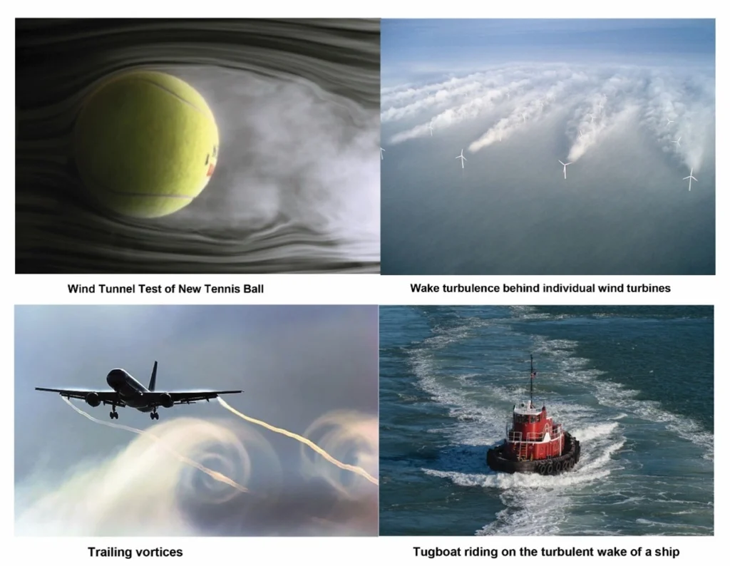
Figure 1- Examples of turbulent dynamics in in real-life and engineering applications

Flow Regime Classification in Fluid Mechanics

If you turn on a faucet (that doesn’t have an aerator or other attachment) at a very low flow rate the water will flow out very smoothly—almost “glass-like.” If you increase the flow rate, the water will exit in a churned-up, chaotic manner (Fig.2). These are examples of how a viscous flow can be laminar or turbulent, respectively. A laminar flow is one in which the fluid particles move in smooth layers, or laminas; a turbulent flow is one in which the fluid particles rapidly mix as they move along due to random three dimensional velocity fluctuations.

Figure 2- Water exiting a tube: (a) laminar flow at low flow rate, (b) turbulent flow at high flow rate, and (c) same as (b) but with a short shutter exposure to capture individual eddies.

Reynolds Number

The transition from laminar to turbulent flow depends on below parameters among other things.

1. Geometry,
2. Surface roughness,
3. Flow velocity,
4. Surface temperature,
5. Type of fluid.

A flow that alternates between being laminar and turbulent is called transitional. The experiments conducted by Osborne Reynolds in the 1880s resulted in the establishment of the dimensionless Reynolds number, Re, as the key parameter for the determination of the flow regime in pipes. Osborne Reynolds built 6-ft. long glass tubes with diameters of 2.68, 1.53, and 0.789 cm with trumpet mouths and passed water through them (Fig.3).

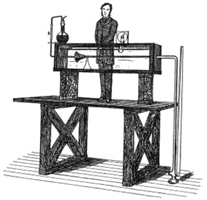
Figure 3- Osborne Reynolds’ original apparatus for demonstrating the onset of turbulence in pipes.

He found that at a low flow rate and/or with a small diameter tube, an injected color streak is seen as a steady streak (Fig.4).

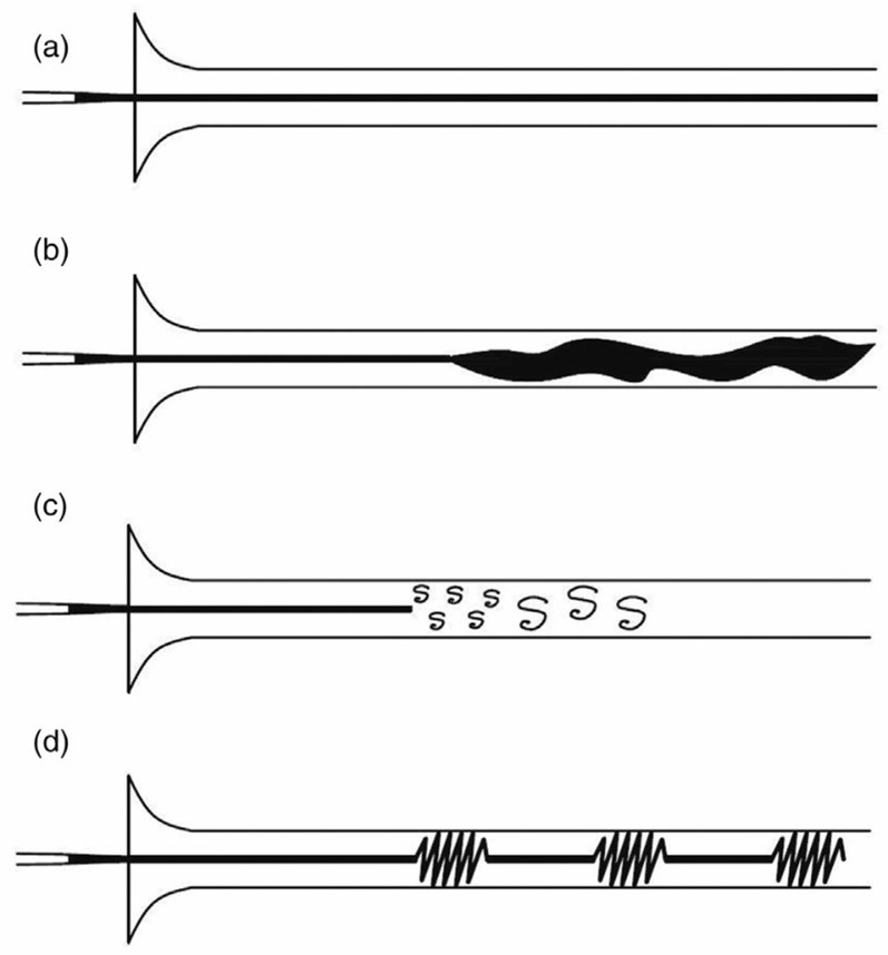
Figure 4- Osborne Reynolds’ experiment on laminar to turbulent flow in a pipe.

In other words, the flow is laminar at low Re where small perturbations are damped out by viscosity. Note that a laminar flow in a smooth long pipe in Fig. 4(a) is named after Poiseuille. At a higher flow rate, the color band shown in Fig. 4 (b) appears to expand and mix with the water. When viewing the tube by the light of an electric spark (Fig. 4 (c)), the mass of color resolves itself into a mass of more or less distinct curls, in which eddies can be seen. In the transitional realm of an intermediate flow rate, as depicted by Fig.4 (d), we see the intermittent character of the flow motion caused by the disturbances, which appear as flashes succeeding each other inside the tube. In other words, we see sporadic bursts of turbulence alternating with laminar flow, indicating a problem with multiple solutions. Consequently, some have approached the origin of turbulence via the bifurcation/chaos method.

After exhaustive experiments in the 1880s, Osborne Reynolds discovered that the flow regime depends mainly on the ratio of inertial forces to viscous forces in the fluid. This ratio is called the Reynolds number and is expressed for internal flow in a circular pipe as shown in the Fig.5.

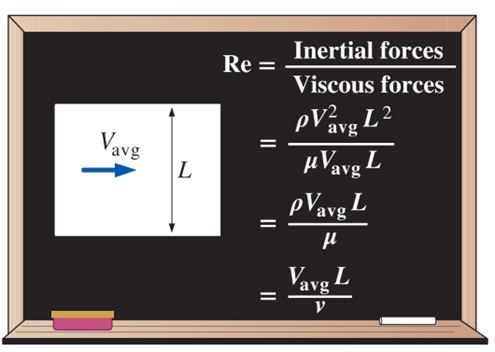
Figure 5- The Reynolds number can be viewed as the ratio of inertial forces to viscous forces acting on a fluid element.

where V_avg = average flow velocity (m/s), D = characteristic length of the geometry (diameter in this case, in m), and 𝜈 = 𝜇/𝜌 = kinematic viscosity of the fluid (m²/s). Note that the Reynolds number is a dimensionless quantity. Also, kinematic viscosity has units m²/s, and can be viewed as viscous diffusivity or diffusivity for momentum.

Flow Regimes for Common Geometrical Configurations

In fluid mechanics, flow behavior significantly depends on the geometry of the object around or through which the fluid moves. Each geometry leads to unique interactions between the fluid and the surface, and thus influences the transition between laminar, transitional, and turbulent flow regimes. These regimes are primarily classified based on the Reynolds number, a dimensionless value that captures the balance between inertial and viscous forces in a flow. Table1 summarizes the typical flow regimes for several common geometries encountered in engineering applications. This classification helps engineers select proper turbulence models in CFD simulations (like in ANSYS Fluent) and optimize mesh quality based on the expected flow behavior.

Table 1- Flow Regimes for Common Geometrical Configurations

Geometry Type	Characteristic Length	Types of Flow Regime
		Laminar	Transitional	Turbulent
Circular Pipe (Internal Flow)	Diameter	Re < 2300	2300 ≤ Re ≤ 4000	Re > 4000
Flat Plate (External Flow)	Plate length	Re < 5 × 10⁵	5 × 10⁵ ≤ Re ≤ ~3 × 10⁶	Re > ~3 × 10⁶
Sphere (External Flow)	Diameter	Re < ~1 × 10⁵	~1 × 10⁵ ≤ Re ≤ ~2 × 10⁵	Re > ~2 × 10⁵
Cylinder (External Flow)	Diameter	Re < ~2 × 10²	~200 ≤ Re ≤ ~2 × 10⁵	Re > ~2 × 10⁵
Airfoil (External Flow)	Chord length	Re < ~5 × 10⁵	—	Re > ~5 × 10⁵
Annular Flow (Pipe with Core)	Hydraulic diameter	Re < 2300	2300 ≤ Re ≤ 4000	Re > 4000

Flow Regimes in Free Convection

In free (natural) convection, the flow regime is determined primarily by the Rayleigh number (Ra), which combines the effects of buoyancy (via the Grashof number) and thermal diffusivity (via the Prandtl number). Unlike forced convection, where the Reynolds number governs flow behavior, free convection relies on Ra to indicate whether the flow is laminar, transitional, or turbulent.

​

​

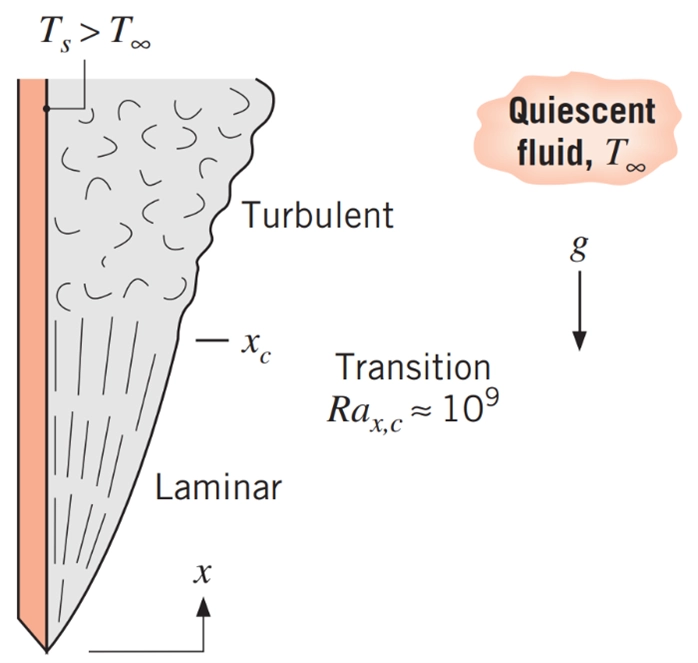
Figure 6- Free convection boundary layer transition on a vertical plate.

Table 2- Flow Regimes in Natural Convection Based on Rayleigh Number

Flow Regime	Rayleigh Number (Ra) Range
Laminar	Ra < 10⁶
Transitional	10⁶ < Ra < 10⁹
Turbulent	Ra > 10⁹

Key Takeaways:

1. The critical Reynolds number varies with geometry and surface conditions.
2. Transition from laminar to turbulent flow is gradual and can be affected by surface roughness, flow disturbances, and inlet conditions.
3. For external geometries, boundary layer behavior plays a major role in determining drag and separation.

Turbulent Flows Characteristics

Because of the complex nature of turbulence, providing a precise definition is often ineffective. Instead, it is more practical to describe turbulence through its key characteristics. In their book “A First Course in Turbulence”, Tennekes and Lumley outline several defining features of turbulent flow, including:

1. Irregularity
2. High diffusivity
3. Occurrence at high Reynolds numbers
4. Fluctuating three-dimensional vorticity
5. Energy dissipation
6. Behavior consistent with the continuum assumption
7. A property of the flow, not the fluid itself

These traits collectively capture the essential nature of turbulent motion.

Irregularity

Turbulent flows are inherently irregular and chaotic, exhibiting complex, unpredictable patterns that vary in space and time. This randomness makes a fully deterministic or exact prediction nearly impossible. As a result, turbulence is often studied using statistical or averaged methods.

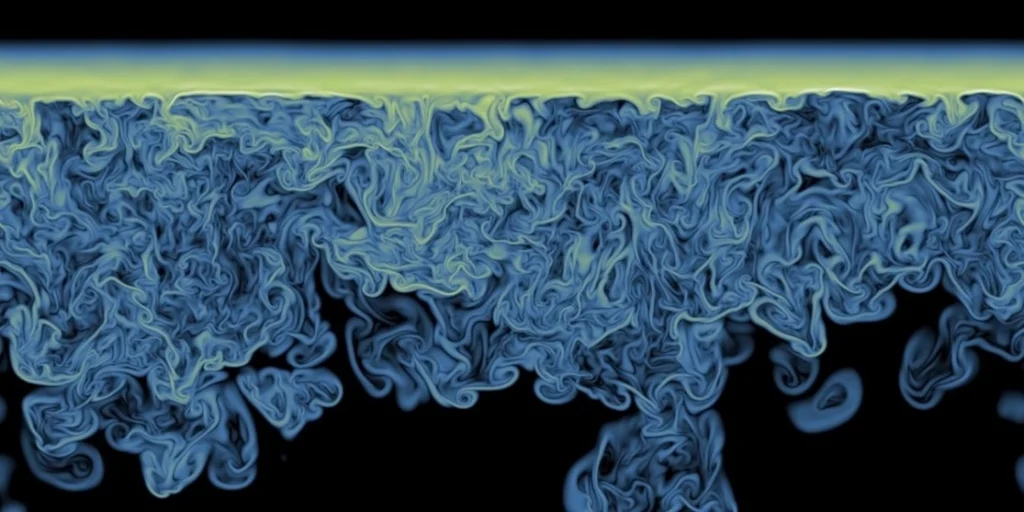
Figure 7- irregularity: a characteristic of turbulent flows.

Diffusivity

 Turbulence significantly enhances the mixing and transport of momentum, heat, and mass. The chaotic eddies promote rapid diffusion across the flow, making turbulent flows far more effective at mixing than laminar ones. If a seemingly random flow does not demonstrate this enhanced mixing, it cannot truly be classified as turbulent.

Figure 8- Diffusivity of Turbulence Lead to Mix Layers

Large Reynolds number

Turbulence typically arises in flows with high Reynolds numbers, where inertial forces dominate over viscous forces. It results from the intricate interplay between non-linear convective effects and viscous dissipation in the Navier–Stokes equations. This interaction leads to instability and ultimately a transition from laminar to turbulent motion.

Figure 9- High Reynolds Number Flow Example

Three-Dimensional vorticity fluctuations.

Turbulent flows are fundamentally three-dimensional and rotational, meaning they contain continuously fluctuating vorticity in all directions. These swirling motions are sustained through mechanisms such as vortex stretching, which cannot occur in purely two-dimensional flows.

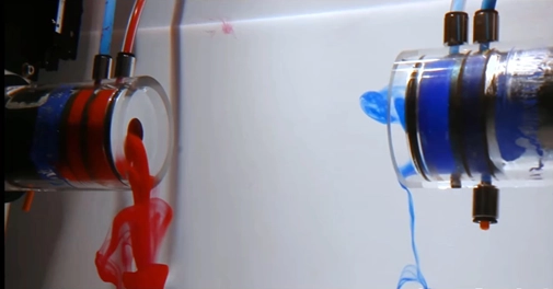
Figure 10- 3D Vorticity Turbulence Structures

Dissipation

Turbulence is dissipative by nature. The kinetic energy introduced at larger scales cascades down to smaller scales, where it is eventually transformed into thermal energy due to viscous effects. Without continuous energy input, turbulent flows gradually decay and revert to a more ordered state.

Figure 11- Energy Dissipation in Turbulence Flow of Water Waves

Continuum

Despite the small-scale structures in turbulence, the flow remains within the continuum regime. Even the tiniest turbulent eddies are much larger than molecular dimensions, allowing classical fluid dynamics to model the behavior effectively using continuum-based equations.

Figure 12- Continuum Assumption in Turbulent Flow in the nature

Feature of a flow, not fluid

Turbulence is not an intrinsic property of the fluid but rather a behavior exhibited by the flow under certain conditions—particularly at high Reynolds numbers. Different fluids may behave similarly under turbulent conditions, highlighting that turbulence depends on flow configuration, not fluid identity.

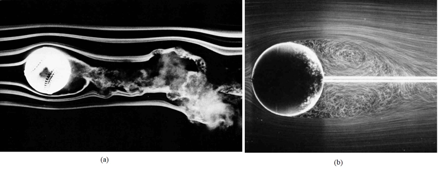
Figure 13- (a) Air flow over a spinning baseball, (b) Water flow over a sphere.

Turbulence Modeling Equations

Both laminar and turbulent flows satisfy the continuity and momentum equations are to be solved for velocity and pressure.

For laminar flow, where there are no random fluctuations, we go right to the attack and solve them for a variety of geometries. For turbulent flow, because of the fluctuations, every velocity and pressure term in equations (1) is a rapidly varying random function of time and space. At present our mathematics cannot handle such instantaneous fluctuating variables. No single pair of random functions V(x, y, z, t) and p(x, y, z, t) is known to be a solution to equations (1). Moreover, our attention as engineers is toward the average or mean values of velocity, pressure, shear stress, and the like in a high-Reynolds-number (turbulent) flow. This approach led Osborne Reynolds in 1895 to rewrite equations (1) in terms of mean or time-averaged turbulent variables. The time mean of a turbulent function u(x, y, z, t) is defined by:

where T is an averaging period taken to be longer than any significant period of the fluctuations themselves. The mean values of turbulent velocity and pressure are illustrated in Fig. 14. For turbulent gas and water flows, an averaging period T=5 s is usually quite adequate.

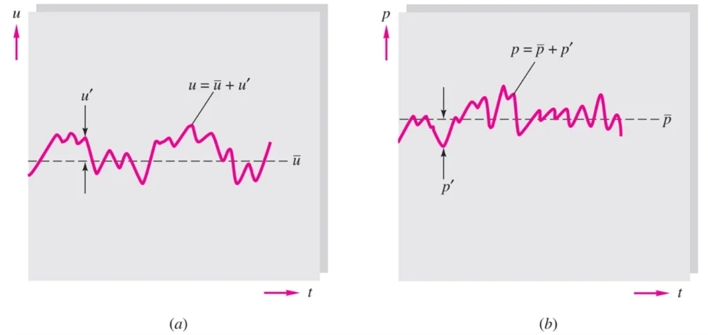
Figure 14- Definition of mean and fluctuating turbulent variables: (a) velocity; (b) pressure.

The fluctuation u′ is defined as the deviation of u from its average value

also shown in Fig. 14. It follows by definition that a fluctuation has zero mean value:

However, the mean square of a fluctuation is not zero and is a measure of the intensity of the turbulence:

Nor in general are the mean fluctuation products such as  and zero in a typical turbulent flow. Reynolds’ idea was to split each property into mean plus fluctuating variables:

Substitute these into Eqs. (1), and take the time mean of each equation. The continuity relation reduces to

which is no different from a laminar continuity relation. However, each component of the momentum equation (1), after time averaging, will contain mean values plus three mean products, or correlations, of fluctuating velocities. The most important of these is the momentum relation in the mainstream, or x, direction, which takes the form

The three correlation terms [latex]−ρu′2,−ρu′v′,−ρu′w′[/latex],  are called turbulent stresses because they have the same dimensions and occur right alongside the newtonian (laminar) stress terms and so on. Actually, they are convective acceleration terms (which is why the density appears), not stresses, but they have the mathematical effect of stress and are so termed almost universally in the literature.

Vorticity, Vortex, and Eddies in Fluid Dynamics

In fluid dynamics, rotational motion plays a fundamental role in shaping how fluids behave under various conditions. Key concepts such as vorticity, vortex, and eddies help us describe and understand different aspects of rotational behavior in flows. While these terms are closely related, each has a distinct meaning and function—vorticity is a mathematical measure of local rotation, a vortex is a physical region where fluid rotates coherently, and eddies are localized swirling motions that often drive mixing. This article explores their definitions, differences, and how they appear in both laminar and turbulent flows.

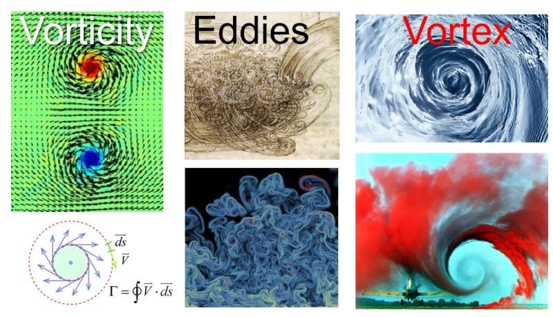
Figure 15- Vorticity, Vortex, and Eddies in Fluid Dynamics

Vorticity, the Mathematical Signature of Rotation

Vorticity is a vector quantity defined as the curl of the velocity field in a fluid. It measures the local rotation of fluid particles about their own center of mass. Even in smooth and orderly laminar flows, vorticity may exist, particularly near solid boundaries or within regions of shear. These rotational tendencies, however, are usually structured and stable. In contrast, turbulent flows contain intense and irregular vorticity distributed throughout the fluid domain. While vorticity is a pointwise and mathematical property, it plays a foundational role in many fluid behaviors, including the formation of larger structures like vortexes and eddies.

Vortex, the Physical Structure of Rotation

A vortex is a coherent and visible region within the fluid where particles revolve around an axis — real or imaginary — in a circular or spiral motion. Vortex formation is influenced by shear layers, solid boundaries, and pressure differences. Vortices can be long-lived and play major roles in phenomena such as drag increase, lift generation, and mixing. In laminar flows, vortexes may exist but tend to be symmetrical, stable, and small in scale. Turbulent flows, on the other hand, generate large, unstable, and complex vortex structures that continuously evolve and interact with each other.

Eddies, the Scales of Swirling Motion

Eddies are swirling motions or circular patterns within a fluid and are generally thought of as smaller or less-coherent than vortexes. They are the dynamic, energy-carrying building blocks of turbulence and exist over a wide range of spatial and temporal scales. Vorticity leads to eddy formation, and clusters of eddies can result in vortex development. While often linked with turbulent flows, eddies can also exist in laminar flows under certain conditions, especially when instabilities or geometric influences are present. In essence, vorticity represents the rotation tendency, eddies are local rotating blobs, and vortexes are sustained flow structures integrating multiple eddies and vorticity regions.

Turbulence models in CFD

Selecting the most suitable turbulence model for your CFD analysis in ANSYS Fluent can be a challenging decision. The choice of turbulence modeling plays a crucial role in the accuracy of simulation results, as the implementation of the model into the numerical scheme significantly influences the outcome; however, the main step involves assessing the Reynolds number, which helps identify the type of fluid flow. While there are types of turbulence modeling methods available to analyze fluid motion, they primarily rely on turbulent viscosity, and no single universal model exists yet. Turbulence models are categorized based on their governing equations and the numerical methods used to compute turbulent viscosity, which serves as the basis for solving turbulence. Among the most widely used turbulence models in CFD are the Reynolds-Averaged Navier-Stokes (RANS) equations and Large Eddy Simulation (LES) methods, which require varying levels of computational resources compared to Direct Numerical Simulation (DNS). Additionally, Unsteady Reynolds-Averaged Navier-Stokes (URANS) is commonly applied in scenarios involving unsteady flows caused by solid body motion or flow separation.

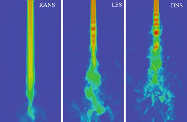
Figure 16- Turbulence models in CFD and their accuracy in flow simulation

There are many turbulence models in use today, including algebraic, one equation, two-equation, and Reynolds stress models. Three of the most popular turbulence models are the k-𝜀 model, and the k-𝜔 model. These so-called two-equation turbulence models add two more transport equations, which must be solved simultaneously with the equations of mass and linear momentum (and also energy if this equation is being used). Along with the two additional transport equations that must be solved when using a two-equation turbulence model, two additional boundary conditions must be specified for the turbulence properties at inlets and at outlets. (Note that the properties specified at outlets are not used unless reverse flow is encountered at the outlet.)

DNS (Direct Numerical Simulation):

Directly solves the Navier-Stokes equations for all turbulence fluctuations without relying on any turbulence model. DNS provides the most accurate results but demands immense computational resources, making it impractical for most engineering applications.

LES (Large Eddy Simulation):

LES acts as an intermediary between DNS and RANS by resolving large-scale turbulent eddies using filtered Navier-Stokes equations, while modeling the effects of small-scale eddies. LES is highly accurate but requires significant computational power.

Figure 17- Large Eddy Simulation (LES) In Hydrocyclones CFD Simulation: Turbulent Flow ANSYS Fluent Example

RANS (Reynolds-Averaged Navier-Stokes):

RANS uses averaged values of variables to simulate both steady-state and dynamic flows. For unsteady flows, URANS (Unsteady RANS) is used, which accounts for turbulence fluctuations caused by motion or separation. RANS methods are computationally efficient and widely applied for most CFD turbulence modeling scenarios.

Figure 18- Dynamic Stall on Pitching Airfoil CFD Simulation: Implementing the SST k-ω turbulence model

Table 3- Comparison of turbulence models for ANSYS Fluent transient flow

Turbulence Model	Accuracy	Computational Cost	Best For
RANS	Moderate	Low	Industrial applications, turbomachinery, general engineering flows
LES (Large Eddy Simulation)	High	High	Vortex shedding, aeroacoustics, race car aerodynamics
DNS (Direct Numerical Simulation)	Very High	Extremely High	Fundamental turbulence research, model validation

Turbulence Models in ANSYS Fluent

The turbulence models in ANSYS Fluent can be categorized based on the main turbulence modeling approaches used in Computational Fluid Dynamics (CFD). These approaches include Reynolds-Averaged Navier-Stokes (RANS), Large Eddy Simulation (LES), Direct Numerical Simulation (DNS), and Hybrid Models. Table 4 shows a detailed categorization:

Table 4- General Classifications of Turbulence Models in ANSYS Fluent

Turbulence Approach	Models in ANSYS Fluent	Applications
RANS	Spalart-Allmaras, k-ε, k-ω, RSM	Industrial flows, steady-state simulations
LES	Standard LES, WALE, Dynamic Smagorinsky	Unsteady flows, large-scale turbulence
DNS	Direct numerical solving (very fine mesh and time stepping)	Research-level simulations, very high accuracy
Hybrid	DES, SAS, PLES	Mixed flows, large eddies with near-wall modeling
Transition	Transition k-kl-ω, Transition SST	Laminar-to-turbulent boundary layer flows

The Fig.19 shows the Viscous Model setup window in ANSYS Fluent, where users select the turbulence model appropriate for their simulation. This section is critical for defining how turbulence is handled in a computational fluid dynamics (CFD) analysis. Here’s a detailed breakdown of the components visible in the picture:

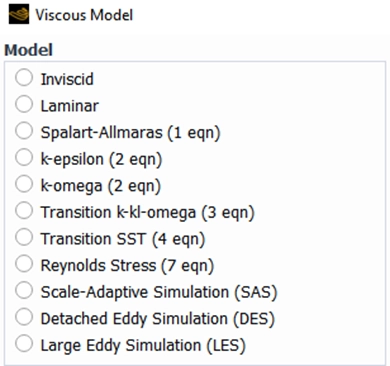
Figure 19- Turbulence Models in the Viscous Model Setup of ANSYS Fluent

Inviscid:

• Assumes no viscosity in the fluid, representing ideal fluid flow.
• Typically used for simplified analyses where viscous effects are negligible.

Laminar:

• Models smooth, orderly flow without turbulence.
• Applicable for low Reynolds number flows or highly viscous fluids.

Spalart-Allmaras (1 Equation):

• A single-equation model designed for external aerodynamic flows, especially in aerospace applications.
• Efficient for boundary layer flows but less accurate for complex turbulence.

k-epsilon (2 Equations):

• One of the most widely used turbulence models.
• Suitable for general-purpose simulations with robust performance in industrial applications.

Variants like Standard, RNG, and Realizable can be selected depending on the type of flow.

k-omega (2 Equations):

• Offers better performance near walls and in boundary layers compared to k-epsilon.
• Commonly used in applications involving adverse pressure gradients.
• Variants include Standardand SST (Shear Stress Transport).

Transition k-kl-omega (3 Equations):

• A three-equation model designed to capture laminar-to-turbulent transition in flows.
• Useful for applications with transitional boundary layers.

Transition SST (4 Equations):

• A four-equation model combining laminar-turbulent transition modeling with SST turbulence modeling.
• Provides higher accuracy for flows undergoing transition.

Reynolds Stress Model (RSM) (7 Equations):

• Solves transport equations for Reynolds stresses directly.
• Used for highly anisotropic flows, such as swirling flows and flows with strong curvature.

Scale-Adaptive Simulation (SAS):

• A hybrid model for unsteady turbulence simulations.
• Automatically adapts the turbulence scale based on flow conditions.

Detached Eddy Simulation (DES):

• Combines RANS near walls with LES for large-scale turbulence in free-stream regions.
• Ideal for flows with complex geometries and dominant turbulence.

Large Eddy Simulation (LES):

• Resolves large eddies directly while modeling smaller ones using subgrid-scale models.
• Provides high accuracy but requires significant computational resources.

Which CFD turbulence model to use?

Each approach to turbulence modeling can be useful depending on the application and the physical quantities of interest. There is a trade-off between computational simplicity and the richness of the information obtained. It is up to the aerodynamicist to choose the appropriate methodology for their needs.  If you’re primarily interested in average flow behavior and computational efficiency, RANS might be a good choice. If you need to capture time-varying phenomena or larger turbulent structures, URANS or LES could be more suitable. DNS remains a valuable research tool for understanding the fundamental physics of turbulence.

Turbulence Modeling in ANSYS Fluent: CFDLAND Tutorial for Turbulent Flow Analysis

At CFDLAND, we are dedicated to helping engineers and researchers master turbulence modeling in CFD for simulating ANSYS Fluent turbulent flow. Whether you’re working in aerospace, automotive, or environmental engineering, we provide expert resources and tutorials to guide you in selecting the best turbulence modeling methods for your application. From reliable approaches like Reynolds-Averaged Navier-Stokes (RANS) to advanced techniques such as Large Eddy Simulation (LES) and Detached Eddy Simulation (DES), our solutions ensure optimized accuracy and efficiency for your CFD simulations.

Our CFD SHOP offers a wide range of ready-to-use simulation resources and custom CFD solutions tailored for turbulent flow analysis. If you’re looking for a turbulent flow ANSYS Fluent example or need personalized assistance with your simulation setup, CFDLAND is here to support you. Visit our Order CFD Project page today to get started and take your turbulence modeling in ANSYS Fluent to the next level!