The Essential Fluid Dynamics Equations

shayan pakravan

Fluid dynamics equations are the mathematical foundations that describe how liquids and gases move and behave under various forces. These essential equations help engineers and scientists solve complex problems involving fluid motion in countless applications across industries. From designing aircraft and ships to optimizing heating systems and understanding blood flow through arteries, these fluid mechanics equations provide crucial insights into physical phenomena.

Contents

In this comprehensive guide, we’ll explore the fundamental equations of fluid dynamics that govern fluid behavior. We’ll break down each equation into simple concepts, explain their physical meaning, and show how they work together to describe complex fluid systems. Whether you’re a student, researcher, or professional engineer, understanding these fluid flow equations is essential for solving real-world problems. The beauty of these governing equations is how they connect mathematical expressions to observable physical behaviors. By mastering these fundamental fluid dynamics equations, you’ll gain powerful tools for analyzing everything from water flowing through pipes to air moving around vehicles.

We will explore the most important fluid dynamics equations, explaining the basic concepts and covering more advanced topics for a well-rounded understanding.

Governing Equations of Fluid Flow and Heat Transfer Dynamics

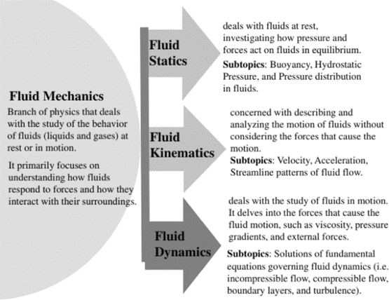
The governing equations of fluid dynamics represent the mathematical expression of three fundamental physical principles: conservation of mass, conservation of momentum, and conservation of energy. These principles form the backbone of all fluid mechanics and allow us to predict fluid behavior across countless scenarios.

Each conservation equation describes how a particular property (mass, momentum, or energy) behaves within a flowing fluid:

Conservation of mass (Continuity Equation): This principle states that mass cannot be created or destroyed within a fluid system. What flows in must equal what flows out, plus any accumulation within the system.
Conservation of momentum (Navier-Stokes Equations): Based on Newton’s second law (F=ma), this principle describes how forces affect fluid motion, accounting for pressure, viscosity, and external forces like gravity.
Conservation of energy (Energy Equation): Following the first law of thermodynamics, this principle tracks how energy transfers and transforms within a fluid, including kinetic energy, potential energy, thermal energy, and work done by forces.

These governing equations form a coupled system of partial differential equations that fully describe fluid behavior when combined with appropriate boundary conditions. While they appear complex mathematically, they simply express how basic physical properties must be conserved during fluid flow. Modern computational fluid dynamics (CFD) software solves these equations numerically to simulate complex flow behaviors that would otherwise be impossible to predict analytically.

The Continuity Equation

The continuity equation represents the mathematical expression of mass conservation in fluid flow. This fundamental principle states that mass cannot be created or destroyed within a fluid system – what goes in must come out, unless it’s stored somewhere in the system.

For a general fluid flow, the continuity equation can be written in differential form as:

$\frac{\partial \rho}{\partial t} + \nabla \cdot (\rho\vec{V}) = 0$

Where:

is the fluid density
is the velocity vector
is time
is the divergence operator

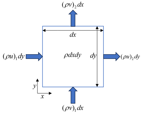
Figure 1: Control volume discretization to examine continuity equation

This equation might look complicated, but it tells us something very straightforward. The first term describes how density changes over time at a specific location. The second term represents how mass flows in and out of a small region through its boundaries.

For incompressible flow (where density remains constant), the continuity equation simplifies to:

$\nabla \cdot \vec{v} = 0$

$\frac{\partial u}{\partial x} + \frac{\partial v}{\partial y} + \frac{\partial w}{\partial z} = 0$

In simpler terms, this means the velocity field has zero divergence – the amount of fluid entering any region must equal the amount leaving that region. This principle has important practical applications, such as explaining why water speeds up when flowing through a narrower pipe section.

For one-dimensional flow in a pipe with varying cross-sectional area, the continuity equation simplifies further to:

A_{1} v_{1} = A_{2} v_{2}

Where $A$ is the cross-sectional area and $v$ is the velocity. This equation directly shows the relationship between flow area and velocity, which is crucial for designing pipe systems, nozzles, diffusers, and many other engineering applications.

The continuity equation works together with the momentum equation and energy equation to form the complete set of governing equations for fluid flow. Understanding this fundamental principle helps engineers analyze and solve problems ranging from simple pipe flows to complex aerodynamics challenges.

Navier-Stokes Equations

The Navier-Stokes equations represent the mathematical expression of momentum conservation in fluid flow. Named after Claude-Louis Navier and George Gabriel Stokes, these equations are essentially Newton’s second law (F=ma) applied to fluid motion. They are among the most important fluid dynamics equations and form the cornerstone of modern fluid mechanics.

Figure 2: George Stokes – the outright father of fluid mechanics

For a viscous, compressible fluid, the Navier-Stokes momentum equation can be written as:

$\rho\frac{D\vec{V}}{Dt} = -\nabla p + \nabla \cdot \tau + \rho\vec{g}$

Where:

$ρ$ is the fluid density
is the velocity vector
is pressure
is the viscous stress tensor
is the gravitational acceleration
$D t$ is the material derivative, representing change following a fluid particle

The left side of the equation represents the acceleration of fluid particles, while the right side accounts for all forces acting on the fluid:

: Pressure forces
: Viscous forces due to fluid friction
: Body forces like gravity

For incompressible flow with constant viscosity, the Navier-Stokes equations can be expanded to:

$\rho\left(\frac{\partial \vec{V}}{\partial t} + (\vec{V} \cdot \nabla)\vec{V}\right) = -\nabla p + \mu\nabla^2\vec{V} + \rho\vec{g}$

Where is the dynamic viscosity of the fluid.

The Navier-Stokes equations are remarkably versatile, describing everything from smoke rising from a cigarette to ocean currents and blood flowing through blood vessels. However, they pose significant mathematical challenges:

They are nonlinear partial differential equations, making analytical solutions impossible for most real-world problems
They exhibit chaotic behavior, meaning tiny differences in initial conditions can lead to completely different outcomes
The existence and smoothness of solutions remain an open mathematical problem (one of the Millennium Prize Problems)

Because of these challenges, engineers often use numerical methods in computational fluid dynamics (CFD) to approximate solutions for practical applications. These numerical approaches discretize the equations and solve them iteratively using computer algorithms. Despite their complexity, the Navier-Stokes equations remain indispensable tools for analyzing fluid flow across virtually every engineering discipline, from aerospace and mechanical engineering to civil and biomedical applications.

The Energy Equation

The energy equation in fluid mechanics expresses the principle of energy conservation within flowing fluids. This fundamental equation tracks how energy transforms and transfers throughout a fluid system, accounting for work done by forces, heat transfer, and changes in various forms of energy.

For a general fluid flow, the complete energy equation can be written as:

$\rho\frac{D}{Dt}\left(e + \frac{V^2}{2} + gz\right) = -\nabla \cdot (p\vec{V}) + \nabla \cdot (k\nabla T) + \nabla \cdot (\tau \cdot \vec{V}) + \rho\vec{f} \cdot \vec{V}$

Where:

is the internal energy per unit mass
is the kinetic energy per unit mass
is the potential energy per unit mass
is the thermal conductivity
is temperature
is the viscous stress tensor
is the body force per unit mass

This comprehensive equation accounts for all energy forms and transfer mechanisms:

The left side represents changes in total energy (internal, kinetic, potential)
The right side includes work done by pressure forces, heat transfer by conduction, work done by viscous forces, and work done by body forces.

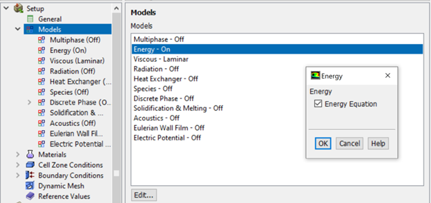
Figure 3: Energy equation enables this way in Ansys Fluent software

For many practical applications, simplified forms of the energy equation are used. For example, in steady, inviscid, incompressible flow along a streamline with no heat transfer, the energy equation reduces to the famous Bernoulli equation:

$\frac{p}{\rho} + \frac{V^2}{2} + gz = \text{constant}$

The energy equation is essential for analyzing numerous engineering systems:

Heat exchangers and thermal management systems
Combustion processes and propulsion systems
Heating, ventilation, and air conditioning (HVAC)
Weather patterns and atmospheric processes
Oceanic currents and environmental flows

Along with the continuity equation and momentum equation, the energy equation completes the set of governing equations that fully describe fluid behavior. Together, these fluid dynamics equations provide engineers with powerful tools for analyzing complex flow problems across virtually every industry and application.

Basic Fluid Dynamics Equations

Several basic fluid dynamics equations derive from the fundamental governing equations we’ve discussed. These simplified relations apply to specific flow conditions and provide practical tools for solving common engineering problems.

Hydrostatic Equation

For fluids at rest or with negligible flow velocity, the Navier-Stokes equations simplify to the hydrostatic equation:

$\frac{dp}{dz} = -\rho g$

This equation shows that pressure in a static fluid increases linearly with depth due to the weight of fluid above. It explains why your ears pop when diving underwater or flying in an airplane.

Streamline Momentum Equation

Along a streamline in steady, inviscid flow, the momentum equation reduces to:

$\frac{dp}{\rho} + VdV + gdz = 0$

This equation relates changes in pressure, velocity, and elevation along a fluid path and forms the basis for Bernoulli’s equation.

Vorticity Equation

The vorticity equation describes how rotation within a fluid evolves:

$\frac{D\vec{\omega}}{Dt} = (\vec{\omega} \cdot \nabla)\vec{V} + \nu\nabla^2\vec{\omega}$

Where is the vorticity vector and $ν$ is the kinematic viscosity. This equation is crucial for understanding turbulent flows, aerodynamic lift, and vortex dynamics.

Stream Function

For two-dimensional, incompressible flow, we can define a stream function $ψ$ that automatically satisfies the continuity equation:

$u = \frac{\partial \psi}{\partial y}, \quad v = -\frac{\partial \psi}{\partial x}$

Where and are velocity components. The stream function simplifies analysis and visualization of 2D flows, as contours of constant $ψ$ represent streamlines.

Potential Function

For irrotational flow (where $\nabla \times V = 0$ ), we can define a velocity potential $ϕ$ :

$\vec{V} = \nabla\phi$

The velocity potential satisfies Laplace’s equation ( $\nabla^{2} ϕ = 0$ ) for incompressible flow, allowing powerful analytical techniques from potential theory to solve flow problems.

These basic fluid dynamics equations provide engineers with practical tools for analyzing specific flow situations without solving the complete Navier-Stokes equations. They form the foundation for understanding both simple and complex fluid behaviors across numerous applications.

Fluid Dynamics Bernoulli Equation

The Bernoulli equation is one of the most widely used and recognizable fluid dynamics equations. Derived from the momentum equation for steady, inviscid, incompressible flow along a streamline, it establishes a fundamental relationship between pressure, velocity, and elevation in fluid flow.

The standard form of the Bernoulli equation is:

$\frac{p}{\rho} + \frac{V^2}{2} + gz = \text{constant}$

Where:

is pressure
$ρ$ is fluid density
$V$ is flow velocity
$g$ is gravitational acceleration
$z$ is elevation

Each term in the Bernoulli equation represents a specific type of energy per unit mass:

$ρ p$ represents pressure energy (or flow work)
$V ^{2}$ represents kinetic energy
$g z$ represents potential energy due to gravity

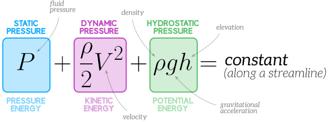
The Bernoulli principle states that as the velocity of a fluid increases, its pressure decreases, and vice versa. This principle explains numerous everyday phenomena:

Lift generation: Airplane wings are designed so air moves faster over the top surface than the bottom, creating lower pressure above and generating lift.
Venturi effect: When fluid flows through a constricted section of pipe, its velocity increases and pressure decreases, explaining how carburetors, atomizers, and spray bottles work.
Pitot tubes: These instruments measure airspeed by comparing stagnation pressure (where velocity is zero) to static pressure, using the Bernoulli equation.

For flow between two points along a streamline, the Bernoulli equation can be written as:

$\frac{p_1}{\rho} + \frac{V_1^2}{2} + gz_1 = \frac{p_2}{\rho} + \frac{V_2^2}{2} + gz_2$

This form is particularly useful for solving practical engineering problems involving pressure and velocity changes in pipe systems, flow through nozzles and orifices, and analyzing aerodynamic forces.

It’s important to remember the Bernoulli equation has limitations:

It applies only to steady, inviscid, incompressible flow along a streamline
It neglects friction, heat transfer, and work done by machines
It cannot be applied across shock waves or in highly turbulent regions

Despite these limitations, the Bernoulli equation remains one of the most powerful and practical tools in fluid mechanics, providing valuable insights into fluid behavior and enabling engineers to solve a wide range of flow problems with remarkable simplicity.

Euler’s Equations

Euler’s equations represent a simplified form of the Navier-Stokes equations for inviscid flow (where viscous effects are neglected). Named after Swiss mathematician Leonhard Euler, these equations provide a powerful tool for analyzing high-speed flows where viscous effects are small compared to inertial forces.

The Euler equations for fluid flow can be written as:

Continuity equation:

$\frac{\partial \rho}{\partial t} + \nabla \cdot (\rho\vec{V}) = 0$

Momentum equation (inviscid form):

$\rho\frac{D\vec{V}}{Dt} = -\nabla p + \rho\vec{g}$

Energy equation (inviscid form):

$\rho\frac{D}{Dt}\left(e + \frac{V^2}{2} + gz\right) = -\nabla \cdot (p\vec{V})$

The key difference between Euler’s equations and the full Navier-Stokes equations is the absence of the viscous stress terms. This simplification makes Euler’s equations more tractable mathematically while still capturing essential flow physics in many applications.

Euler’s equations are particularly valuable for analyzing:

High Reynolds number flows: When inertial forces dominate viscous forces, making viscous effects negligible except in boundary layers
External aerodynamics: Flow around aircraft, missiles, and vehicles at high speeds where the flow can be treated as inviscid outside thin boundary layers
Shock waves and supersonic flow: Capturing discontinuities and wave propagation in compressible flow
Potential flow: Under certain conditions, Euler’s equations can be further simplified to potential flow theory, enabling powerful analytical solutions

For steady flow along a streamline, Euler’s equation reduces to:

$\frac{dp}{\rho} + VdV + gdz = 0$

Integrating this equation yields the famous Bernoulli equation discussed earlier.

While Euler’s equations provide valuable insights into many fluid dynamics problems, they have important limitations:

They cannot predict skin friction or flow separation
They fail to capture boundary layer development
They cannot account for viscous dissipation of energy

Despite these limitations, Euler’s equations remain a cornerstone of theoretical fluid dynamics and provide the foundation for numerous computational methods used in aerospace engineering, weather prediction, and other fields requiring analysis of complex fluid flows.

Darcy-Weisbach Equation

The Darcy-Weisbach equation is a fundamental relation in fluid mechanics that calculates pressure or head loss due to friction in pipe flows. Named after Henry Darcy and Julius Weisbach, this practical equation is essential for designing pipe systems, analyzing flow distribution networks, and sizing pumps and valves.

The standard form of the Darcy-Weisbach equation is:

$h_f = f\frac{L}{D}\frac{V^2}{2g}$

Where:

$h_{f}$ is the head loss due to friction (energy loss per unit weight of fluid)
$f$ is the Darcy friction factor (dimensionless)
$L$ is the pipe length
$D$ is the pipe diameter
$V$ is the average flow velocity
$g$ is the gravitational acceleration

In terms of pressure drop, the equation can be written as:

$\Delta p = f\frac{L}{D}\frac{\rho V^2}{2}$

The Darcy friction factor ( $f$ ) depends on:

Whether the flow is laminar or turbulent
The pipe’s relative roughness (, where $ε$ is the absolute roughness)
The Reynolds number of the flow ()

For laminar flow (), the friction factor is simply:

$f = \frac{64}{Re}$

Where:

f = Darcy friction factor (dimensionless)
Re = Reynolds number

For turbulent flow ( $R e > 4000$ ), the friction factor is typically determined using the Colebrook equation or its explicit approximations like the Swamee-Jain equation:

$f = \frac{0.25}{\left[\log_{10}\left(\frac{\epsilon/D}{3.7} + \frac{5.74}{Re^{0.9}}\right)\right]^2}$

The Moody diagram provides a graphical method for determining the friction factor based on Reynolds number and relative roughness.

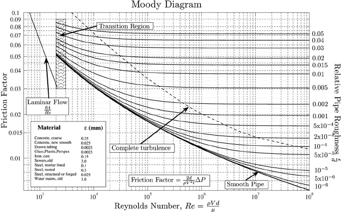
Figure 4: The Moody diagram – Reynolds number Vs. Friction factor

The Darcy-Weisbach equation is derived from the Navier-Stokes equations by applying them to pipe flow and making appropriate simplifications. It represents a practical application of the fundamental fluid dynamics equations to real engineering problems.

Unlike empirical formulas like the Hazen-Williams equation, the Darcy-Weisbach equation has several advantages:

It’s dimensionally homogeneous and works with any consistent set of units
It applies to all fluids, not just water
It accounts for temperature effects through fluid viscosity
It’s theoretically sound, being derived from fundamental principles

Engineers use the Darcy-Weisbach equation daily to design water distribution systems, industrial piping networks, HVAC systems, and many other applications involving fluid flow in pipes and conduits. Understanding and applying this equation is essential for predicting pressure losses and ensuring efficient fluid transportation in countless engineering systems.

Conclusion

The essential fluid dynamics equations we’ve explored form the mathematical foundation for understanding and predicting how fluids behave in countless real-world applications. These powerful governing equations help engineers and scientists solve complex flow problems across virtually every industry and field of study.

Let’s review the key fluid mechanics equations we’ve covered:

The continuity equation ensures mass conservation in flowing fluids, showing that mass cannot be created or destroyed within a fluid system.
The Navier-Stokes equations apply Newton’s second law to fluids, describing how forces affect fluid motion through momentum conservation.
The energy equation tracks how energy transforms and transfers throughout a fluid system, following the principle of energy conservation.
The Bernoulli equation provides a simplified relationship between pressure, velocity, and elevation for steady, inviscid flow along a streamline.
Euler’s equations offer a valuable simplification of the Navier-Stokes equations by neglecting viscous effects, useful for analyzing high-speed and potential flows.
The Darcy-Weisbach equation calculates pressure losses due to friction in pipe flows, essential for designing real-world fluid systems.

These fundamental fluid dynamics equations work together to describe everything from water flowing through pipes to air moving around aircraft. While they may appear complex mathematically, they simply express how basic physical properties (mass, momentum, and energy) must be conserved during fluid motion.

Modern engineering relies heavily on these equations through computational fluid dynamics (CFD) software, which solves them numerically to simulate complex flow behaviors. This allows engineers to design more efficient vehicles, create better medical devices, optimize energy systems, and address environmental challenges without expensive physical prototyping.

Understanding these fluid mechanics equations provides valuable insight into both natural phenomena and engineered systems. Whether you’re studying laminar flow in blood vessels, turbulent flow around buildings, or heat transfer in industrial processes, these governing equations form the foundation of analysis and design.

By mastering these essential fluid dynamics equations, you gain powerful tools for solving real-world problems across disciplines ranging from aerospace and mechanical engineering to environmental science and biomedical applications. The mathematical language of fluids truly unlocks our ability to understand, predict, and control the flow of liquids and gases that surrounds us every day.

The Essential Fluid Dynamics Equations

Governing Equations of Fluid Flow and Heat Transfer Dynamics

The Continuity Equation

Navier-Stokes Equations

The Energy Equation

Basic Fluid Dynamics Equations

Hydrostatic Equation

Streamline Momentum Equation

Vorticity Equation

Stream Function

Potential Function

Fluid Dynamics Bernoulli Equation

Euler’s Equations

Darcy-Weisbach Equation

Conclusion

Related Blogs

What is a Dimensionless Number?

Conservation of Mass in Fluid Mechanics

Energy Conservation Equation

What is Computational Fluid Dynamics (CFD)?

Leave a Comment Cancel Reply

CFDLand