
The ANSYS Fluent Axisymmetric modeling approach is a powerful technique used to reduce computational time and resources when dealing with geometries that are symmetric around an axis as it drastically reduces the mesh size and simulation time. Common examples include nozzles, pipes, and cylindrical reactors. This article provides an in-depth look at the 2D axisymmetric method in ANSYS Fluent, its applications, and how it integrates with ANSYS Workbench for streamlined Computational fluid dynamics (CFD) analysis. We’ll explore key concepts such as axisymmetric swirl, and how to use the axisymmetric axis model. Whether you are modeling a nozzle in ANSYS Fluent, a pipe, or any other symmetric component, this guide offers both theoretical insight and a practical tutorial for setup.
What’s the difference between Symmetric and Axisymmetric models?
In CFD, symmetric and axisymmetric refer to different types of geometric and flow symmetries. A symmetric model displays mirror symmetry across a plane, meaning one side is a reflection of the other. In contrast, axisymmetric specifically pertains to systems that exhibit symmetry around a central axis, allowing for the simplification of three-dimensional problems into two-dimensional analyses. While axisymmetric modeling is best suited for problems with circular or cylindrical symmetry, symmetric modeling works well for planar mirror-like geometries. The figure 1 compares (a) a 3D cylindrical model reduced to an axisymmetric model by taking a 2D cross-section along the radial and axial directions, and (b) a 2D flow domain simplified to a symmetric model by simulating only half of the geometry due to mirror symmetry along the centerline.
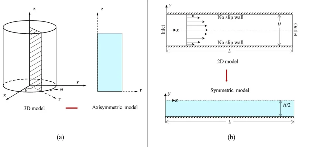
Figure 1- Comparison of axisymmetric (a) [1] and symmetric (b) modeling approaches for geometry simplification in CFD simulations
ANSYS Fluent Axisymmetric
In ANSYS Fluent, the axisymmetric model simplifies the analysis of flows where the geometry and flow field exhibit symmetry about an axis, typically the z-axis. This assumption reduces the problem from three dimensions (3D) to two dimensions (2D), significantly improving computational efficiency without sacrificing accuracy in many cases. The model is particularly useful for simulating flows in pipes, nozzles, diffusers, and other axisymmetric geometries. The figure 2 depicts a cylindrical slice representing an axisymmetric case in fluid dynamics.
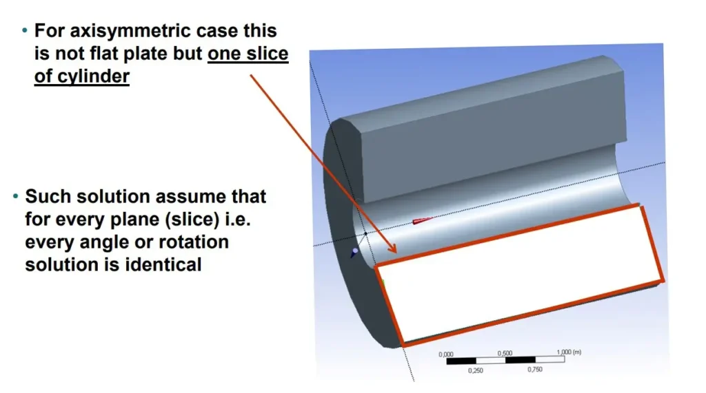
Figure 2- Axisymmetric model representation: a case study for simulation by ANSYS Fluent
What is Axisymmetric Swirl?
The assumption of axisymmetric implies that there are no circumferential gradients in the flow, but that there may be non-zero circumferential velocities. Axisymmetric swirl refers to a flow condition in which a fluid moves around a central axis while exhibiting uniform rotational motion, characterized by a consistent angular velocity. In this type of flow, properties such as velocity, pressure, and temperature remain constant with respect to the azimuthal angle ( ), allowing for a two-dimensional representation in cylindrical coordinates. The figure 3 illustrates a cylindrical flow system with an axis of symmetry, depicting a region where fluid experiences swirl characterized by the angular velocity ω.
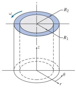
Figure 3- Laminar viscometric flow of liquid in annular gap between vertical concentric cylinders [2]
Another example of axisymmetric swirl Fluent is the figure 4. This picture depicts a cylindrical flow domain illustrating an axisymmetric swirl configuration, with labeled inflow and outflow directions along the z-axis, a symmetry axis at the center, and a shaded area indicating the region of interest for analyzing the swirling flow.
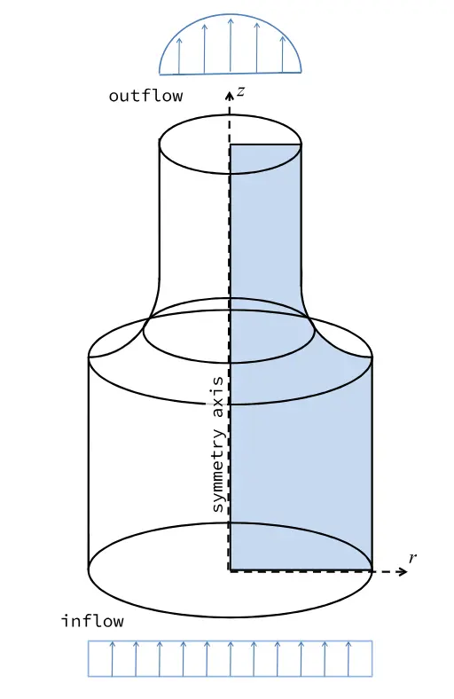
Figure 4- Axisymmetric swirl method at ANSYS Fluent for a Cylindrical Domain
Axisymmetric Swirl – When to Use
Use Axisymmetric Swirl when you have tangential motion, like in:
- Cyclone separators
- Rotating flows
- Swirling jets
- Vortex tubes
But the flow is still symmetric in θ (no variation in θ).
Governing Equations in Axisymmetric Model
In axisymmetric coordinates (Fig.5), the governing equations are adapted to reflect the cylindrical symmetry around a central axis (typically the -axis), which simplifies the mathematical treatment of problems in such configurations.
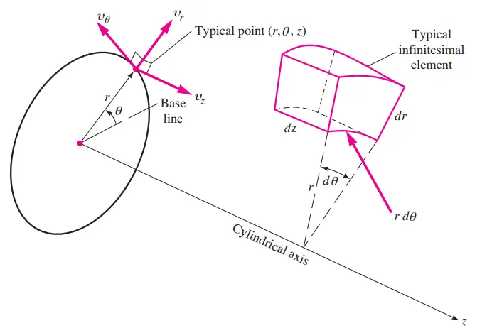
Figure 5- Definition sketch for the cylindrical coordinate system [3]
Before axisymmetric assumption
In cylindrical coordinates the general form of the governing equations for incompressibility flow are as follows:
- Incompressible continuity equation:

- r-component of the incompressible Navier–Stokes equation:
![\rho \left(\frac{\partial u_r}{\partial t} + u_r\frac{\partial u_r}{\partial r} + \frac{u_\theta}{r}\frac{\partial u_r}{\partial \theta} - \frac{u_\theta^2}{r} + u_z\frac{\partial u_r}{\partial z}\right) = -\frac{\partial P}{\partial r} + \rho g_r + \mu\left[\frac{1}{r}\frac{\partial}{\partial r}\left(r\frac{\partial u_r}{\partial r}\right) - \frac{u_r}{r^2} + \frac{1}{r^2}\frac{\partial^2 u_r}{\partial \theta^2} - \frac{2}{r^2}\frac{\partial u_\theta}{\partial \theta} + \frac{\partial^2 u_r}{\partial z^2}\right]](https://cfdland.com/wp-content/ql-cache/quicklatex.com-b5ea13e6073bf589334d65c9adea7661_l3.png "Rendered by QuickLaTeX.com")
- θ-component of the incompressible Navier–Stokes equation:
![\rho \left(\frac{\partial u_\theta}{\partial t} + u_r\frac{\partial u_\theta}{\partial r} + \frac{u_\theta}{r}\frac{\partial u_\theta}{\partial \theta} + \frac{u_ru_\theta}{r} + u_z\frac{\partial u_\theta}{\partial z}\right) = -\frac{1}{r}\frac{\partial P}{\partial \theta} + \rho g_\theta + \mu\left[\frac{1}{r}\frac{\partial}{\partial r}\left(r\frac{\partial u_\theta}{\partial r}\right) - \frac{u_\theta}{r^2} + \frac{1}{r^2}\frac{\partial^2 u_\theta}{\partial \theta^2} + \frac{2}{r^2}\frac{\partial u_r}{\partial \theta} + \frac{\partial^2 u_\theta}{\partial z^2}\right]](https://cfdland.com/wp-content/ql-cache/quicklatex.com-b14db3763a055127df7a417ebd110ea3_l3.png "Rendered by QuickLaTeX.com")
· z-component of the incompressible Navier–Stokes equation:
![\rho \left(\frac{\partial u_z}{\partial t} + u_r\frac{\partial u_z}{\partial r} + \frac{u_\theta}{r}\frac{\partial u_z}{\partial \theta} + u_z\frac{\partial u_z}{\partial z}\right) = -\frac{\partial P}{\partial z} + \rho g_z + \mu\left[\frac{1}{r}\frac{\partial}{\partial r}\left(r\frac{\partial u_z}{\partial r}\right) + \frac{1}{r^2}\frac{\partial^2 u_z}{\partial \theta^2} + \frac{\partial^2 u_z}{\partial z^2}\right]](https://cfdland.com/wp-content/ql-cache/quicklatex.com-6ed34b2f62eae30a313ae67dd965d8c5_l3.png "Rendered by QuickLaTeX.com")
where is the density of the fluid, is the pressure, g is acceleration of gravity, and is the dynamic viscosity. In addition, , are the velocity components in the radial, azimuthal, and axial directions, respectively.
Equations after axisymmetric assumption
If the problem involves flow through a round pipe, nozzle, or any geometry that is rotationally symmetric, it is efficient to model it using the axisymmetric approach in ANSYS Fluent. This allows a 3D domain described in cylindrical coordinates to be simplified into a 2D computational domain in the plane by assuming that all physical quantities are independent of the angular direction , i.e.,

With the axisymmetric assumption, the governing equations in ANSYS Fluent simplify because the derivative with respect to the angular coordinate is dropped.
- The flow is symmetric in the θ-direction, i.e.

- If the fluid moves around a central axis, the azimuthal (swirl) velocity component is
- If we do not have in this way the governing equations will be reduced to 2D while representing a rotationally symmetric three dimensional problem.
How to use axisymmetric model in ANSYS Fluent?
Modeling axisymmetric fluid flow in ANSYS Fluent (with or without swirl) involves a few specific settings and considerations during preprocessing, setup, and solution. Here’s a clear guide to get you started:
Step1: Create 2D Geometry
Use a section of the geometry in the r–z plane (usually with vertical axis as z). The geometry must be axisymmetric around the x=0 line (the z-axis). For example, for pipe flow, draw the pipe’s radial cross-section.
Step2: Mesh the Geometry
Mesh the 2D section in your preprocessor (e.g., ANSYS Meshing or ICEM CFD). Make sure the boundary along is aligned with the axis of symmetry.
Step3: Set Up in Fluent
Go to: Setup → General → Solver (Fig.6)
Set the solver 2D Space: Axisymmetric (or Axisymmetric Swirl if your problem involves swirl motion)
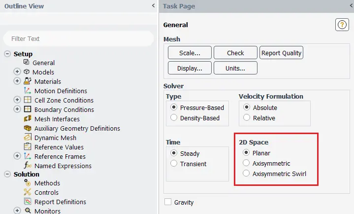
Figure 6- The schematic of general setting in ANSYS Fluent
Step4: Define Boundary Conditions
- Carefully define: Axis (at r = 0): Set boundary type as axis (Fig.7)
- Set Wall, inlet, outlet as per usual
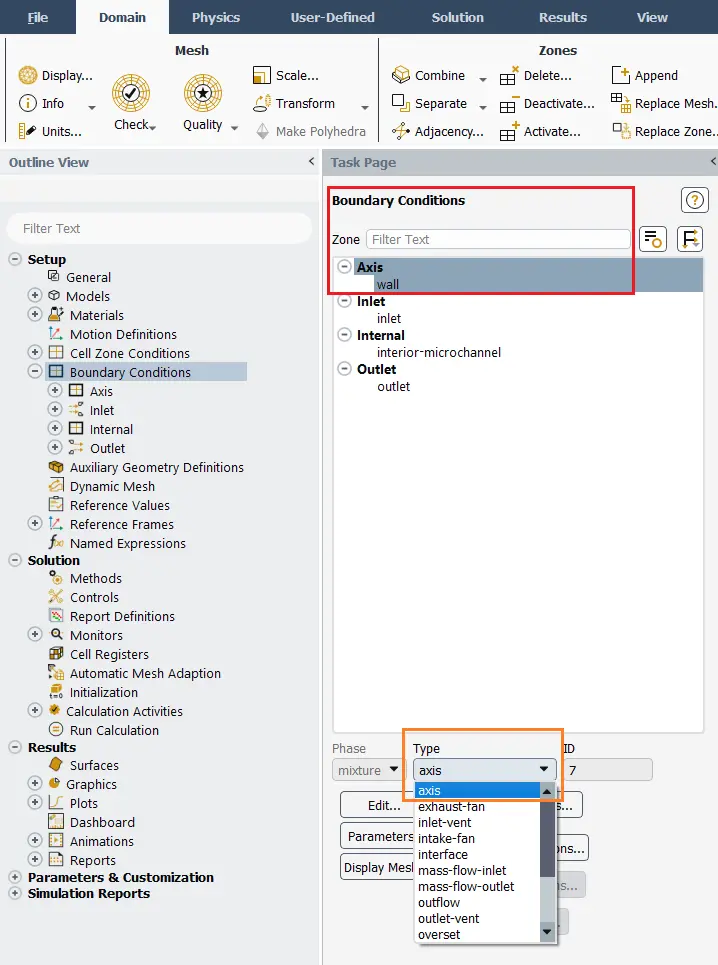
Figure 7- How should Define Boundary Conditions for Axisymmetric models
Step4: Post-Processing
Results are 2D but interpreted as revolved around the axis. You can visualize:
- Velocity vectors in the plane
- Contours of , and swirl velocity if existing
- Streamlines, pressure, temperature, etc.
- Use “Contours of Swirl Velocity” to see the azimuthal flow patterns.
2D axisymmetric tutorial
At CFD LAND, we offer a variety of 2D Axisymmetric Tutorials designed to help you master the essentials of CFD simulations, for instance, high-pressure water jet nozzles which are essential in industries like cutting, cleaning, and hydraulic mining. Our ANSYS Fluent Training will teach you how to model and analyze high-pressure water nozzle jets using this efficient ANSYS 2D axisymmetric method (Fig.8).
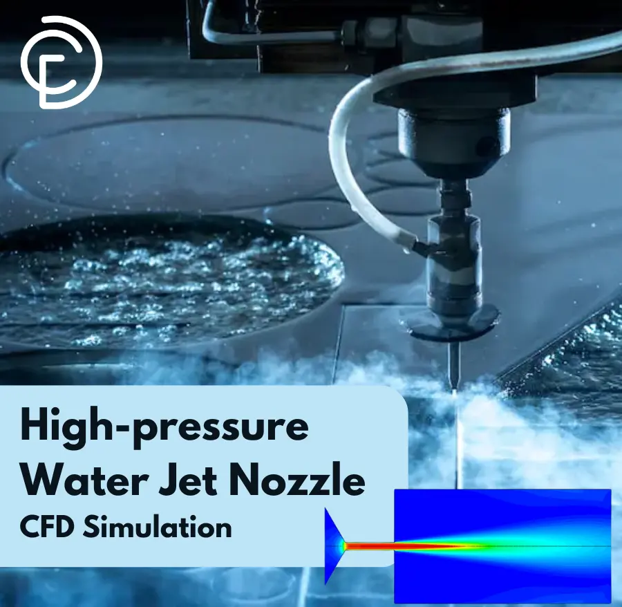
Figure 8- High-pressure Water Jet Nozzle CFD Simulation, 2D axisymmetric tutorial
Axisymmetric ANSYS Workbench also can be utilized for orifice cavitation which occurs when fluid passing through a narrow opening experiences a pressure drop, forming vapor bubbles that collapse downstream. In our ANSYS Fluent workflow, we use 2D axisymmetric ANSYS mechanical approach to model the orifice geometry in ANSYS Design Modeler, reducing computational costs while ensuring accurate results in cavitating flow simulations (Fig.9).

Figure 9- Orifice Cavitating Flow Using Cavitation Model CFD Simulation – 2D Axisymmetric Tutorials
What are the main requirements for an axisymmetric analysis?
- Geometric Symmetry: The physical domain must exhibit symmetry about a central axis.
- Flow Conditions: It is important to note that while the assumption of axisymmetry implies that there are no circumferential gradients in the flow, there may still be non-zero swirl velocities.
- Mesh Quality: The mesh should be refined near boundaries and in regions with expected high gradients.
- Boundary Conditions Must Be Axisymmetric: Any inlet, outlet, or wall condition must not vary with the angular direction (θ). All boundary conditions must also be symmetric about the axis. For example, you can’t apply different temperatures or velocities at different angular positions.
Conclusion
The ANSYS Fluent Axisymmetric modeling approach provides a highly efficient method for analyzing fluid flows in geometries that exhibit symmetry around a central axis. By simplifying three-dimensional problems into two-dimensional analyses, this technique significantly reduces computational time and resource requirements while maintaining accuracy for a wide range of applications, including nozzles, pipes, and cylindrical reactors. The article has outlined the key differences between symmetric and axisymmetric models, highlighted the importance of axisymmetric swirl in specific flow conditions, and detailed the governing equations and procedural steps for effective implementation in ANSYS Fluent. With proper geometric symmetry, appropriate boundary conditions, and a well-structured mesh, users can leverage this powerful modeling approach to enhance their CFD analyses and achieve reliable results in various engineering scenarios.
FAQs
- What is axisymmetric analysis in CFD?
Axisymmetric analysis refers to the simulation of fluid flow in geometries that exhibit symmetry around a central axis. This allows for the reduction of a three-dimensional problem to a two-dimensional one, simplifying the computational process while preserving the essential flow characteristics.
- What are the benefits of using axisymmetric modeling?
The primary benefits include reduced computational time and resources, simplified mesh generation, and the ability to focus on specific flow features without the complexities of three-dimensional modeling.
- What types of applications are suitable for axisymmetric analysis?
Axisymmetric analysis is ideal for applications such as flow through pipes, nozzles, cylindrical reactors, and other systems where the geometry is symmetric around a central axis.
- What are the key requirements for conducting an axisymmetric analysis?
Key requirements include geometric symmetry, and appropriate boundary conditions with no circumferential gradients in the flow.
- What is the significance of axisymmetric swirl in fluid flow?
Axisymmetric swirl refers to the rotational motion of fluid around the central axis.
- Can axisymmetric analysis be used for unsteady flows?
Yes, axisymmetric analysis can be applied to both steady and unsteady flows.
Reference
[1] Zhang, H., Li, J., Li, H., Ye, H., Zhang, H., & Zheng, Y. (2023). A coupled axisymmetric peridynamics with correspondence material model for thermoplastic and ductile fracture problems. International Journal of Fracture, 244(1), 85-111.
[2] Pritchard, Philip J., and John W. Mitchell. Fox and McDonald’s introduction to fluid mechanics. John Wiley & Sons, P.204, 2011.
[3] White, Frank M. University of Rhode Island. Fluid mechanics. P.234, (2011).