ANSYS Fluent Transient Simulation

Kiarash Kord

Transient Simulation in ANSYS Fluent is essential for capturing time-dependent fluid dynamics, unlike steady-state simulations, which assume constant flow properties. Since most natural flows are transient, using ANSYS Fluent transient simulation provides accurate modeling of vortex shedding, rotating machinery, and multiphase flows. Although steady solutions are computationally less expensive, transient analysis is necessary when time-dependent effects cannot be ignored. This study explores the fundamental principles of transient simulations, highlighting key differences from steady-state simulations and their essential applications. It provides a step-by-step guide for configuring and running simulations, including transient thermal analysis, compressible flow modeling, and visualization techniques using animations and data tables. Engineers and researchers can utilize this guide to improve transient CFD analysis and optimize design processes effectively.

Contents

Steady State vs. Transient Simulation in ANSYS Fluent

Steady-State Simulation assumes that flow variables remain constant over time and are suitable for problems where transients die out quickly. On the other hand, Transient Simulation, captures the evolution of flow characteristics, making it ideal for flows with oscillations, shocks, or time-dependent sources. The Fig.1 compares velocity magnitude (v) for flow over a cylinder, showing (a) steady-state flow with smooth, symmetric velocity distribution and (b) ANSYS Fluent transient flow simulation with unsteady vortex shedding and alternating high and low velocity regions in the wake.

Figure 1- The steady state and a snapshot of the transient flow regime[1]

The decision between steady and transient modeling depends on the problem requirements, computational cost, and the need for time-resolved data. Table 1 shows a general comparison between steady-state and transient simulations

Table 1- A general overview comparing steady-state and transient simulations.

Aspect	Steady-State	Transient
Definition	Assumes flow variables are constant over time.	Resolves time-dependent changes in flow variables.
Computational Cost	Lower due to fewer iterations.	Higher due to time-stepping and iterative convergence.
Applications	Suitable for stable flows (e.g., laminar pipe flow).	Required for unsteady flows (e.g., vortex shedding, shock waves).
Post-Processing	Easier to analyze.	Requires time-series data analysis.

Transient Simulation in ANSYS Fluent

Transient simulations in ANSYS Fluent are essential for capturing unsteady flow phenomena such as vortex shedding and shock waves. If you’re looking to enhance your understanding of these complex flows, our specialized CFD simulation tutorials and training materials provide hands-on guidance. From Vortex Induced By Cylinder Vibration (Dynamic Mesh) (Fig.2) to Vortex-Based Fluidic Oscillator CFD Simulation (Fig.3), our step-by-step tutorials help engineers and researchers master transient analysis. Additionally, our Film Cooling Improvement by Vortex Generator CFD Simulation (Fig.4) offers insights into optimizing thermal performance using advanced CFD techniques. Whether you’re a beginner or an expert, these ANSYS Fluent simulations will elevate your skills in transient flow analysis.

Figure 2- ANSYS Fluent Tutorial: Vortex Induced By Cylinder Vibration (Dynamic Mesh) CFD Simulation

Figure 3- ANSYS Fluent Training: CFD Simulation of a Vortex-Based Fluidic Oscillator

Origins of Unsteady Flow

Understanding these origins of unsteady flow helps in accurately modeling transient simulations in CFD applications. Overall, unsteady flow can arise from both natural instabilities and external forces, leading to time-dependent – fluid behavior.

Natural Unsteadiness: Unsteady flow occurs due to the inherent growth of fluid instabilities or a non-equilibrium initial state. Examples include:

Kelvin–Helmholtz Instability – Formation of vortices due to velocity differences in adjacent fluid layers.
Natural Convection Flows – Driven by buoyancy forces in heated fluids.
Turbulent Eddies – Multi-scale vortex structures in turbulent flows.
Fluid Waves – Includes gravity waves, shock waves, and surface waves.

Fig. 4 presents ANSYS Fluent transient simulation example for different types of case studies: Kelvin–Helmholtz Instability (a)[2], Natural Convection Flows (b)[3], Turbulent Eddies (c)[4], and Fluid Waves (d).

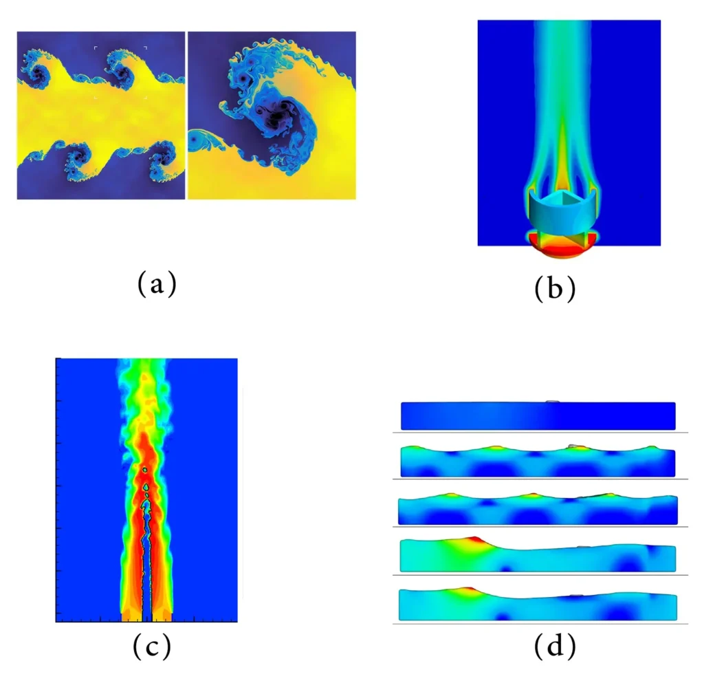
Figure 4- Examples of natural unsteadiness requiring transient simulation

Forced Unsteadiness: External factors such as time-dependent boundary conditions or varying source terms induce unsteady behavior. Examples include:

Pulsing Flow in a Nozzle – Periodic pressure variations causing oscillatory motion.
Rotor-Stator Interaction in Turbomachinery – Unsteady pressure fluctuations due to rotating and stationary components.

Figure 5 illustrates ANSYS Fluent transient simulation example for (a) a pulsing flow in a nozzle and (b)[5] a rotor-stator interaction in turbomachinery.

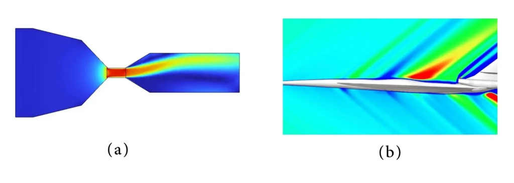
Figure 5- Examples of forced unsteadiness requiring transient simulation

ANSYS Fluent transient formulation

Transient Flow Modeling in ANSYS Fluent involves solving time-dependent equations that govern the motion, heat transfer, and interactions of fluids. Unlike steady-state simulations, ANSYS Fluent transient formulation captures changes in flow properties over time, making it crucial for analyzing unsteady phenomena such as vortex shedding, turbulence, and compressible flows. The mathematical foundation of Governing Equations for transient fluid dynamics is based on the Navier-Stokes equations, which include:

Continuity Equation (Mass Conservation):

$\frac{\partial \rho}{\partial t} + \nabla \cdot (\rho\mathbf{v}) = 0$

Momentum Equations (Newton’s Second Law):

$\frac{\partial (\rho\mathbf{v})}{\partial t} + \nabla \cdot (\rho\mathbf{v}\mathbf{v}) = -\nabla p + \nabla \cdot (\tau) + \rho\mathbf{g}$

Energy Equation (Heat Transfer):

$\frac{\partial(\rho E)}{\partial t} + \nabla \cdot (\mathbf{v}(\rho E + p)) = \nabla \cdot (k\nabla T) + \Phi$

Where:
- ρ = density
- v = velocity vector
- p = pressure
- τ = stress tensor
- E = total energy
- k = thermal conductivity
- Φ = dissipation function
To solve these equations numerically, time discretization is applied:
- Implicit Method: Stable for larger time steps, solving equations at the next time step simultaneously.
- Explicit Method: Solves equations sequentially but requires small time steps for stability.

Key Considerations in Transient Simulations

When performing ANSYS Fluent transient flow simulations, several critical factors must be carefully considered to ensure numerical stability, accuracy, and computational efficiency. These factors include:

Time step selection
Courant number
Turbulence modeling
Boundary conditions

Below is a detailed explanation of each consideration, along with an example to illustrate its impact.

I) Time Step Selection

The time step size (Δt) is crucial in ANSYS Fluent transient flow simulations. It must be small enough to accurately capture transient effects, yet large enough to minimize computational cost.

II) Courant number

The Courant-Friedrichs-Lewy (CFL) number ensures numerical stability in ANSYS Fluent transient flow simulations:

$C = \frac{u\Delta t}{\Delta x}$

where:

u = velocity magnitude,
Δx = grid spacing,
Δt= time step.

For explicit solvers, C≤1 is required for stability, whereas implicit solvers can handle higher values.

III) Turbulence Modeling in Transient Simulations

Turbulence modeling is a crucial aspect of ANSYS Fluent transient flow simulations, as it helps predict time-dependent vortex structures, energy dissipation, and flow instabilities. Depending on the required accuracy and computational cost, different turbulence models can be used. Fig. 6 and Table 2 present a comparison of turbulence models used in ANSYS Fluent for simulating transient flow.

Figure 6- Turbulence models in CFD and their accuracy in flow simulation [6]

Table 2- Comparison of turbulence models for ANSYS Fluent transient flow

Turbulence Model	Accuracy	Computational Cost	Best For
URANS (Unsteady RANS)	Moderate	Low	Industrial applications, turbomachinery, general engineering flows
LES (Large Eddy Simulation)	High	High	Vortex shedding, aeroacoustics, race car aerodynamics
DNS (Direct Numerical Simulation)	Very High	Extremely High	Fundamental turbulence research, model validation

IV) ANSYS Fluent Transient Boundary Conditions

Boundary conditions must be time-dependent to accurately model unsteady flows.

Considerations:

Use time-dependent velocity profiles for inlets.
Ensure pressure variations at outlets are realistic

V) ANSYS Fluent Transient Convergence

Ensuring ANSYS Fluent transient convergence is crucial for obtaining stable and reliable results.

Best Practices:

Use PISO (Pressure-Implicit with Splitting of Operators) for faster convergence.
Monitor residuals and flow parameters over time.
Adjust time step size dynamically if convergence issues arise.

ANSYS Fluent transient thermal analysis

Transient thermal analysis calculates temperature variations and other thermal parameters that change over time. This type of analysis is crucial for various heat transfer applications, including:

Heat treatment processes
Thermal management in electronic packaging
Nozzle temperature distribution
Engine block cooling and heating cycles
Pressure vessel thermal performance

The governing equation for the heat conduction through a solid is given by:

$k(\frac{\partial^2 T}{\partial x^2} + \frac{\partial^2 T}{\partial y^2} + \frac{\partial^2 T}{\partial z^2}) + q = \rho c\frac{\partial T}{\partial t}$

Figure 7 presents the ANSYS Fluent transient thermal analysis of a Solar Still (Distiller). Upon ordering this product from our website, you will be provided with a geometry file, a mesh file, and an in-depth Training Video that offers a step-by-step training on the simulation process.

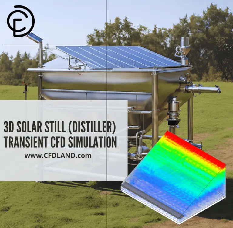
Figure 7- Thermal analysis of a notebook cooling system

How to Model Transient Flows in ANSYS Fluent

Modeling transient (unsteady) flows in ANSYS Fluent requires setting up time-dependent simulations to capture flow variations over time. Here, there are some points you should consider for modeling transient flows in ANSYS Fluent.

Point1: Enable Transient (Unsteady) Solver

To enable the unsteady solver: Go to General → Time → Transient to enable time-dependent calculations (fig.8).

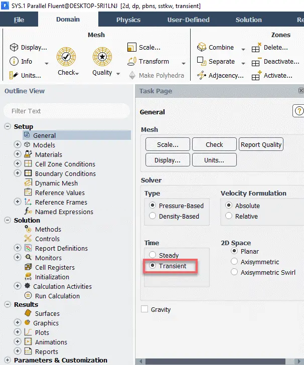
Figure 8- Enabling the unsteady solver

Point2: Report Definition section

One of the most important aspects of time-dependent simulation is the output results. If you intend to extract a time-dependent graph of a variable, it is better to define it in the Report Definition section at the very beginning (Fig.9).

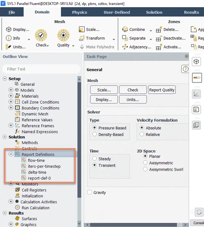
Figure 9- Enabling the Report Definitions in time-dependent simulations

Point3: Set Up Time Step Size

Choose an appropriate time step size (Δt) based on the flow characteristics and Courant number (typically, CFL<1). Keep in mind that convergence must be achieved at each time step. You can use the following formula to determine the time step.

$\Delta t = \frac{\text{Min (Cell Size)}}{\text{Velocity}}$

Given the cell size used in meshing and the inlet velocity in the fluid domain, the appropriate time step for your simulation can be obtained. In addition to selecting the time step size, you must also specify the number of time steps to define the total simulation duration (Fig.8). For example, if you set this value to 100 and your time step size is 0.01, multiplying them will give you the total simulation time, which in this case is 1 second.

Simulation Time = 0.01*100 = 1 second

Finally, after defining the time step size and number of time steps, you need to select the number of iterations per time step (Fig.11). By setting this value, ANSYS Fluent will solve the governing flow equations for the specified number of iterations at each time step. If convergence is achieved in fewer iterations than the defined limit, the solver will proceed to the next time step. It is recommended to set a high number of iterations to ensure that the simulation reaches convergence at each time step.

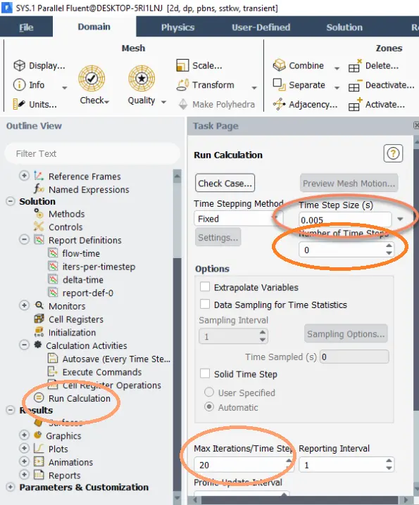
Figure 10- Set up the Run Calculation setting

Point4: Choose Solver Type

Select Pressure-Based or Density-Based solver. For most incompressible transient flows, pressure-based solver is recommended. For high-speed compressible flows, use the density-based solver (see fig.11).

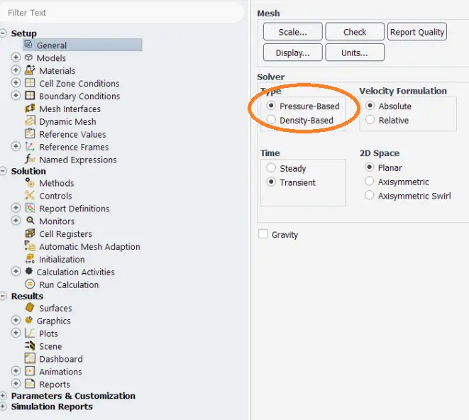
Figure 12- Selecting types of solver

Poin5: Choose a Turbulence Model (if applicable)

For turbulent flows, select a turbulence model like k-ε, k-ω SST, or LES (Large Eddy Simulation) for higher accuracy in transient cases.

Poin6: Set Up Boundary Conditions

Define appropriate inlet, outlet, and wall boundary conditions. For transient flows, you may need time-dependent boundary conditions (e.g., varying velocity or pressure at the inlet).

Point7: Initialize the Flow Field

Use Hybrid Initialization or initialize the flow field based on steady-state results to provide a starting point for the transient simulation.

Post-Processing

Use ANSYS Fluent’s post-processing tools to visualize flow features such as velocity contours, pressure fields, streamlines, and vortex shedding. Extract time-dependent data (e.g., lift and drag coefficients, temperature variations, or flow oscillations).

I) ANSYS Fluent Transient Animation

Enable Animation:

Go to Solution > Calculation Activities > Graphics and Animations and create an animation (Contour, Vector, etc.).

Set Parameters: Choose a variable, set frame frequency, and define view settings.
Run & Export: Run the simulation, preview the animation, and export as AVI/MP4.

II) ANSYS Fluent Transient Table

In transient simulations, extracting numerical data in table format helps analyze time-dependent results. You can create a table in ANSYS Fluent using:

Report Definitions: Go to Results > Reports, define monitors for tracking variables.
Export Data: Use Monitors & Reports to save results in CSV format.
Fluent Console: Use text commands (e.g., report summary) to generate tables.

Conclusion

In this study we provide a comprehensive guide to transient flow modeling in ANSYS Fluent, emphasizing its importance for capturing time-dependent fluid dynamics compared to steady-state simulations. It explains the key principles of transient analysis, including the mathematical foundation (Navier-Stokes equations), critical considerations like time step selection, Courant number, turbulence modeling, and boundary conditions. The guide outlines step-by-step instructions for setting up transient simulations, such as enabling the unsteady solver, defining report outputs, selecting solvers, and initializing the flow field. Additionally, it highlights practical applications like vortex shedding, rotating machinery, and transient thermal analysis, supported by examples of natural and forced unsteadiness. Post-processing techniques, including animations and data extraction, are also detailed to analyze time-dependent results effectively. This article can be considered as a valuable resource for engineers and researchers to model unsteady flows, optimize designs, and improve simulation accuracy.

FAQs

What is transient simulation in ANSYS Fluent?

Transient simulation captures time-dependent fluid dynamics, unlike steady-state simulations that assume constant flow properties. It is essential for modeling unsteady phenomena like vortex shedding, turbulence, and rotating machinery.

What are the origins of unsteady flow?

Unsteady flow can arise from natural instabilities (e.g., Kelvin-Helmholtz instability, turbulent eddies, natural convection) or external forces (e.g., pulsing flow, rotor-stator interactions).

What are the key considerations for transient simulations?

Critical factors include selecting an appropriate time step size, maintaining a stable Courant number, choosing the right turbulence model, applying time-dependent boundary conditions, and ensuring convergence.

How do you select the time step size for transient simulations?

The time step size is determined based on the Courant number (CFL<1) and flow characteristics, ensuring it is small enough for accuracy but large enough to minimize computational cost.

What turbulence models are suitable for transient simulations?

Common models include:

URANS: Moderate accuracy, low cost, suitable for industrial applications.
LES: High accuracy, high cost, ideal for vortex shedding and aeroacoustics.
DNS: Very high accuracy, extremely expensive, used for fundamental turbulence research.

What are common applications of transient simulations?

Applications include vortex shedding, shock waves, rotating machinery, multiphase flows, and transient thermal analysis.

How do you ensure convergence in transient simulations?

Use methods like PISO (Pressure Implicit with Splitting of Operators), monitor residuals, and adjust time step size dynamically if convergence issues arise.

Reference

[1] T. Breiten, K. Kunisch, and L. Pfeiffer, “Feedback stabilization of the two-dimensional Navier–Stokes equations by value function approximation,” Applied Mathematics & Optimization, vol. 80, pp. 599-641, 2019.

[2] V. Springel, C. Klingenberg, R. Pakmor, T. Guillet, and P. Chandrashekar, “EXAMAG: Towards Exascale Simulations of the Magnetic Universe,” in Software for Exascale Computing-SPPEXA 2016-2019, 2020: Springer International Publishing, pp. 331-350.

[3] https://www.aerotak.dk/da/naturligkonvektion, ed.

[4] https://web.stanford.edu/group/pitsch/Research/LES.htm, ed.

[5] https://semiengineering.com/accelerating-speed-and-accuracy-in-aeroacoustic-predictions/, ed.

[6] K. Velten, W. Lubitz, and A. Hopf, “Simulation of airflow within horticulture high-tunnel greenhouses using open-source CFD software,” PhD thesis, 02 2018.

Leave a Comment Cancel Reply