Fluid Mechanics CFD Simulation

What is Fluid Mechanics?

Fluid mechanics is the branch of physics that deals with the mechanics of fluids (liquids, gases, and plasmas) and the forces on them. A fluid is a substance that cannot resist a shear stress by a static deflection and deforms continuously as long as the shear stress is applied. We can see the difference between solid and fluid behavior in Fig. 1 If we place a specimen of either substance between two plates (Fig.1 (a)) and then apply a shearing force F, each will initially deform (Fig.1 (b)); however, whereas a solid will then be at rest (assuming the force is not large enough to go beyond its elastic limit), a fluid will continue to deform ((Fig.1 (c)), (Fig.1 (d)), etc.) as long as the force is applied. Note that a fluid in contact with a solid surface does not slip—it has the same velocity as that surface because of the no-slip condition, an experimental fact.

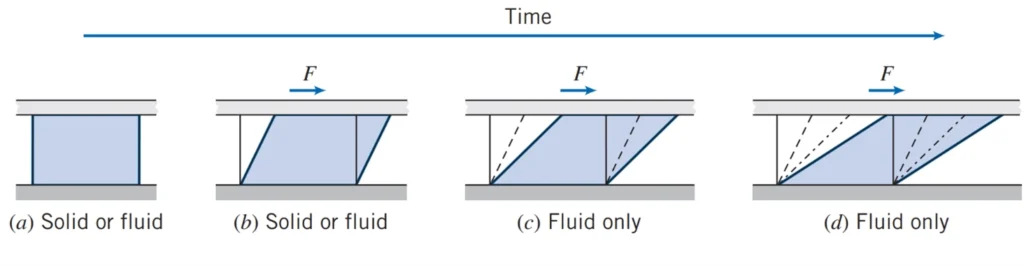
Figure 1- Difference in behavior of a solid and a fluid due to a shear force

Application of CFD in Fluid Mechanics

Fluid mechanics can be divided into fluid statics or the study of fluids at rest; and fluid dynamics or the study of the effect of forces on fluid motion. Fluid mechanics has a wide range of applications, including mechanical engineering, chemical engineering, geophysics, astrophysics, and biology. Fluid mechanics, especially fluid dynamics, is an active field of research with many problems that are partly or wholly unsolved. Commercial code based on numerical methods is used to solve the problems of fluid mechanics. The principles of these methods are developed by computational fluid dynamics (CFD), a modern discipline that is devoted to this approach to solve the aforementioned problems.

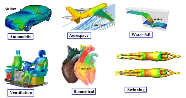
Figure 2- Application of Computational Fluid dynamics (CFD) in Fluid Mechanics

Fundamental Concepts of Fluid Mechanics

Understanding the fundamental concepts of fluid mechanics is essential for anyone working with Computational Fluid Dynamics. Whether you’re simulating airflow over a car or analyzing liquid cooling in electronics and so on, concepts like the no-slip condition, boundary layer, Reynolds number, etc. form the backbone of accurate and reliable simulations. The following introduces key principles that every CFD user should know to better understand fluid behavior and improve simulation results.

The No-Slip Condition

The no-slip condition is a fundamental principle in fluid mechanics stating that a fluid in contact with a solid surface has zero relative velocity—meaning the fluid “sticks” to the wall. This assumption is crucial in CFD simulations, as it directly affects the velocity profile near boundaries, determines the shear stress distribution, and influences heat transfer rates. Accurately applying the no-slip condition ensures realistic modeling of boundary layers and flow behavior in practical engineering problems.

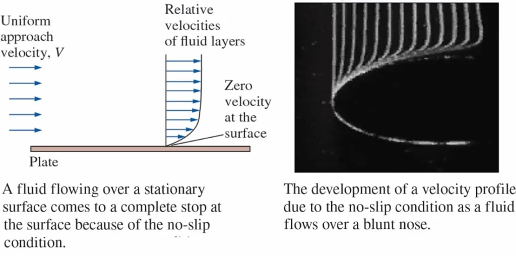
Figure 3- The no-slip Condition in Fluid Mechanics

Boundary Layer

The boundary layer is a thin region adjacent to a solid surface where viscous forces dominate and the fluid velocity transitions sharply from zero at the wall (due to the no-slip condition) to the free-stream value.  Outside this region, the fluid moves almost unaffected by the wall. This layer is crucial in fluid mechanics as it governs the drag experienced by objects, influences flow separation and transition to turbulence, and must be accurately resolved in CFD simulations—especially when using turbulence models like k-ε, k-ω, or LES—to ensure realistic and reliable results.

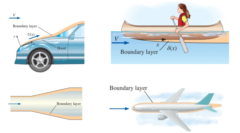
Figure 4- The Boundary Layer Region in Fluid Mechanics

System and Control Volume

In fluid mechanics and thermodynamics, a system refers to a defined quantity of matter or a specific region in space selected for analysis. Everything outside the system is called the surroundings, and the boundary is the interface between them. A closed system (or control mass) contains a fixed amount of matter and does not allow mass to cross its boundary, though energy (heat or work) may. A control volume, on the other hand, is an open system where both mass and energy can cross the boundary. Control volumes are used to analyze devices like compressors, turbines, and nozzles, where fluid flows in and out. Boundaries in control volumes can be fixed or moving, and choosing an appropriate control volume simplifies the analysis significantly.

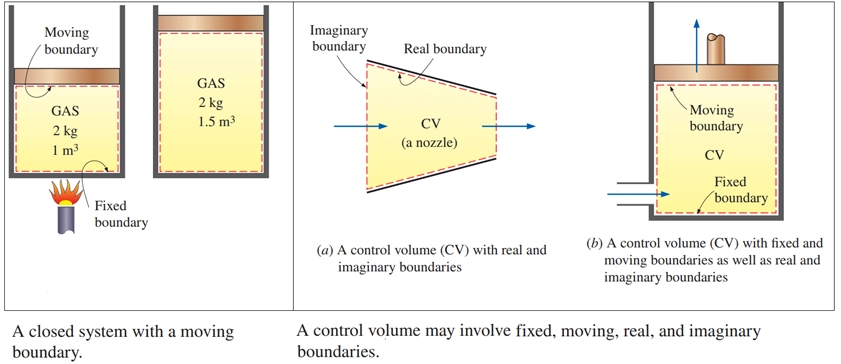
Figure 5-System and Control Volume Differences in Fluid Mechanics

Surface Tension

Surface tension is a phenomenon commonly observed in everyday life—such as water droplets forming on leaves, soap bubbles floating in the air, or mercury rolling like a ball on glass. In these cases, the liquid surface behaves like a stretched elastic membrane. This behavior arises from the cohesive forces between liquid molecules, which pull inward and cause the surface to minimize its area. The force per unit length acting along the surface is known as surface tension (𝜎ₛ), typically measured in N/m. It can also be interpreted as surface energy—the amount of energy required to increase a liquid’s surface area by one square meter. Surface tension explains why droplets tend to adopt spherical shapes, as spheres have the minimum surface area for a given volume.

Figure 6- Surface Tension in Fluid Mechanics

Capillary Effect

The capillary effect is a result of surface tension and occurs when a liquid rises or falls in a narrow tube-or capillary-inserted into the fluid. This phenomenon is driven by the interaction between cohesive forces within the liquid and adhesive forces between the liquid and the solid surface. For example, water rises in a thin glass tube because it “wets” the surface, forming an upward-curved meniscus, while mercury, which does not wet glass, forms a downward-curved meniscus and slightly descends. The capillary effect explains everyday observations like the upward movement of kerosene in a lamp wick or how water travels through the small vessels in plants.

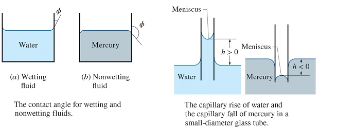
Figure 7- Capillary Effect in Fluid Mechanics

Flow Separation

Flow separation occurs when a fluid can no longer follow the contour of a surface due to an adverse pressure gradient-often caused by high velocity or sharp curvature. This leads the fluid to detach from the surface. A common analogy is a car losing contact with the road on a sharp curve or when speeding over a hill-just as the wheels lift off, the fluid separates from the surface. After separation, a low-pressure region forms behind the object, called the separated region, where flow recirculates or reverses. This increases pressure drag. Downstream of this region is the wake, where the flow remains disturbed and turbulent before gradually returning to normal. Separation is influenced by factors like: Reynolds number, Surface shape, and Turbulence intensity. Understanding and controlling flow separation is critical in improving aerodynamic and hydrodynamic performance.

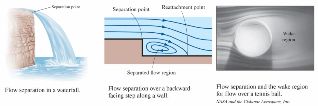
Figure 8- Flow Separation in Fluid Mechanics

Classification of Continuum Fluid Mechanics

There is a wide variety of fluid flow problems encountered in practice, and it is usually convenient to classify them on the basis of some common characteristics to make it feasible to study them in groups. There are many ways to classify fluid flow problems, and here we present some general categories. Fig.9 presents the various classifications of fluid flow in fluid mechanics. Each classification highlights a fundamental aspect of fluid behavior, helping to distinguish different flow regimes and analyze fluid motion in diverse engineering and scientific applications.

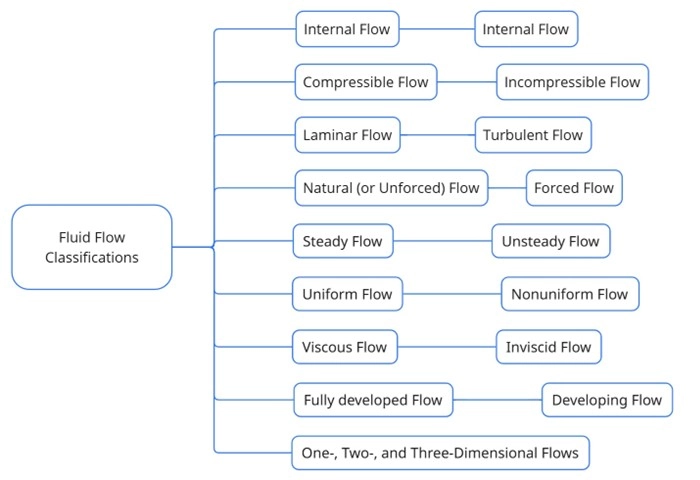
Figure 9- Possible Classification of Continuum Fluid Mechanics.

Internal versus External Flow

Fluid flow can be categorized as internal or external based on the presence of surrounding boundaries. When a fluid moves within enclosed spaces like pipes or ducts, it is considered internal flow, as the fluid is completely confined by solid walls. On the other hand, external flow refers to situations where the fluid moves over surfaces without being fully enclosed—such as air passing over a flat plate, a ball, or a pipe exposed to wind. When liquid flows through a channel that is not completely filled and has a free surface—like rivers or open canals—it is known as open-channel flow. In internal flows, viscous forces affect the entire flow, while in external flows, these effects are mostly limited to the boundary layer regions near surfaces and the wake areas behind objects.

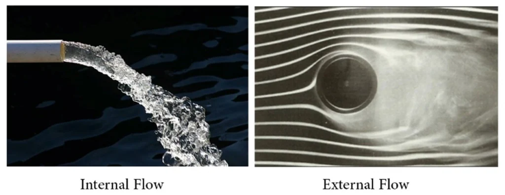
Figure 10- Internal versus External Flow in Fluid Mechanics

Compressible versus Incompressible Flow

A flow is classified as compressible or incompressible based on how much the fluid’s density changes during motion. In incompressible flow, the density remains nearly constant throughout the fluid, making it a useful approximation in many practical cases—especially for liquids. This means that the volume of any fluid element does not change as it moves. In contrast, in compressible flow, density variations are significant, which is typically the case in high-speed gas flows. Usually, all fluids experience slight changes in density with pressure changes. Whether a fluid is assumed to be compressible or incompressible depends on the context and the level of precision required by the engineer or scientist.

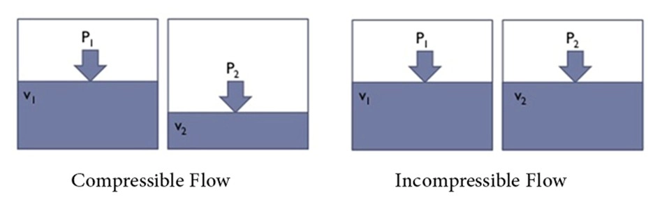
Figure 11- Compressible versus Incompressible Flow in Fluid Mechanics

Laminar versus Turbulent Flow

Some fluid flows are smooth and orderly, while others are more chaotic. The well-organized fluid motion involving smooth layers is known as laminar flow. The term laminar refers to the movement of adjacent fluid particles in layers, or “laminae.” Fluids with high viscosity, like oils, tend to exhibit laminar flow at low velocities. In contrast, turbulent flow is marked by irregular fluid motion and velocity fluctuations, commonly occurring at higher velocities. Low-viscosity fluids such as air usually show turbulent behavior at high speeds. When a flow shifts between laminar and turbulent behavior, it is referred to as transitional flow. Osborne Reynolds’ experiments in the 1880s led to the development of the dimensionless Reynolds number (Re), which serves as a key criterion for identifying the flow regime in pipes.

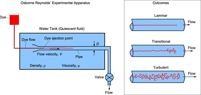
Figure 12- Laminar versus Turbulent Flow in Fluid Mechanics

Natural (or Unforced) versus Forced Flow

Fluid flow is classified as either natural or forced based on how the motion is initiated. In forced flow, the fluid is driven over a surface or through a pipe by external devices such as a pump or a fan. In contrast, natural flow occurs due to natural forces, such as buoyancy, where warmer (and therefore lighter) fluid rises while cooler (and heavier) fluid sinks. A common example is in solar hot-water systems, where the thermosiphon effect is used to eliminate the need for pumps by positioning the water tank above the solar collectors.

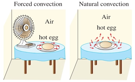
Figure 13- The cooling of a boiled egg by forced and natural convention

Steady vs. Unsteady Flow

In engineering, the concepts of steady and uniform are commonly used, so it’s important to clearly distinguish between them. A flow is considered steady if its properties—such as velocity, pressure, and temperature—do not change at a given location over time. If these properties vary with time, the flow is termed unsteady. Meanwhile, the term uniform refers to a situation where a property remains constant over a specific region in space, regardless of time. Although unsteady and transient are often used interchangeably, they do not mean exactly the same thing. In fluid mechanics, unsteady refers to any time-dependent flow, while transient is usually reserved for flows that are in the process of developing toward a steady state. For example, when a rocket engine is ignited, the pressure and flow characteristics initially change before eventually stabilizing—this phase is described as transient. If an unsteady flow fluctuates in a regular pattern around a constant average, it is referred to as periodic flow.

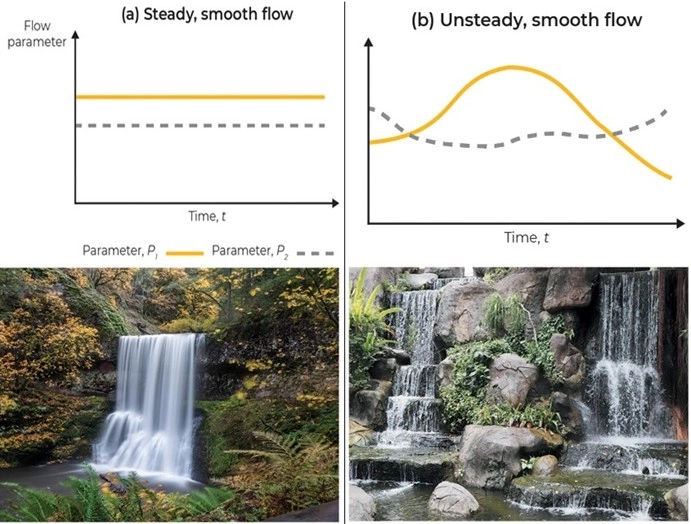
Figure 14- Steady vs. Unsteady Flow in Fluid Mechanics

Uniform versus Nonuniform Flow

In uniform flow, fluid properties such as velocity, pressure, and temperature remain constant at every point in space. A typical example is the test section of a wind tunnel, which is carefully designed to maintain as uniform a flow as possible. Still, near the tunnel walls, the flow becomes nonuniform due to the no-slip condition and the formation of a boundary layer, as previously discussed.

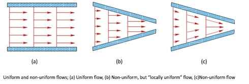
Figure 15- Uniform versus Nonuniform Flow in Fluid Mechanics

In engineering, it’s a common practice to assume flow is uniform in ducts, pipes, and around inlets or outlets- even when it’s not entirely accurate- to simplify calculations.

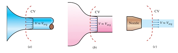
Figure 16- Examples of inlets or outlets in which the uniform flow approximation is reasonable: (a) the well-rounded entrance to a pipe, (b) the entrance to a wind tunnel test section, and (c) a slice through a free water jet in air.

Viscous vs. Inviscid Flow

In fluid mechanics, viscous flow refers to real flows where viscosity plays a role in fluid motion. In contrast, inviscid flow doesn’t mean the fluid has no viscosity- instead, it refers to regions where viscous forces are so small that they can be ignored compared to pressure or inertial forces. Although friction and viscous stresses still exist in these areas, they often cancel out, resulting in no significant net viscous force. That’s why some call it “frictionless flow,” though this can be misleading. To avoid confusion, it’s better to say “regions with negligible viscous effects” rather than “inviscid flow.” Finally, this discussion illustrates the very significant difference between inviscid flow (μ=0) and flows in which viscosity is negligible but not zero (μ→0).

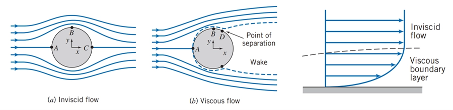
Figure 17- Qualitative picture of incompressible flow over a sphere.

In fluid mechanics, developing flow refers to the entrance region of a pipe or duct where fluid properties are still adjusting, the velocity profile is evolving, and effects like velocity and shear stress change along the flow direction; after the entrance length, the flow becomes fully developed, meaning the velocity profile and other properties remain constant along the pipe, making calculations for pressure drop and heat transfer more straightforward compared to the complex, variable behavior seen in the developing region. The fully developed flow in a circular pipe is one-dimensional since the velocity varies in the radial r-direction but not in the angular θ- or axial z-directions.

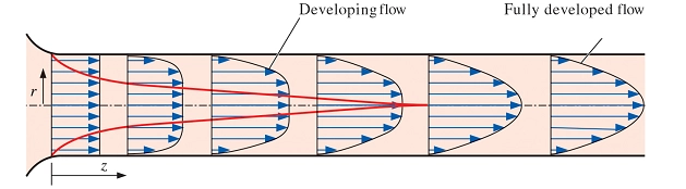
Figure 18- Developing Flow vs. Fully Developed Flow

One-, Two-, and Three-Dimensional Flows

A flow is classified as one-, two-, or three-dimensional based on how many spatial coordinates are needed to describe its velocity field. In general, real-world flows are inherently three-dimensional since velocity may vary with all three coordinates (e.g., x,y,z in Cartesian or r,θ,z in cylindrical systems). However, in many practical situations, if the variation of velocity in one or more directions is negligible, the flow can be approximated as one- or two-dimensional to simplify analysis. For instance, in the entrance region of a pipe, the flow velocity varies significantly in both the radial and axial directions, making it two-dimensional. But farther downstream, once the flow becomes fully developed, velocity only varies with the radial coordinate and remains constant along the pipe’s axis and angular direction, allowing it to be modeled as one-dimensional in cylindrical coordinates. Importantly, the dimensionality also depends on the choice of coordinate system, and simplifying assumptions are valid as long as they do not significantly affect the accuracy of results.

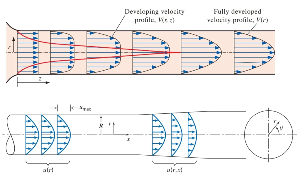
Figure 19- Examples of one- and two-dimensional flows, based on different coordinates.

Newtonian and Non-Newtonian Fluids

In fluid mechanics, fluids are categorized based on how they respond to shear stress. Newtonian fluids exhibit a linear relationship between shear stress and strain rate — their viscosity remains constant regardless of the applied force. Common examples include water, air, gasoline, and mineral oils. On the other hand, non-Newtonian fluids have a viscosity that changes with shear rate or stress. This means their flow behavior is more complex and cannot be described by a single viscosity value. Examples of non-Newtonian fluids include blood, ketchup, toothpaste, liquid plastics, and slurries. These fluids are widely studied in engineering, biomedical applications, and industrial processes due to their unique flow characteristics. Understanding the differences between Newtonian and non-Newtonian fluids is essential for accurate fluid flow modeling, CFD simulation, and the design of mechanical systems where such fluids are present.

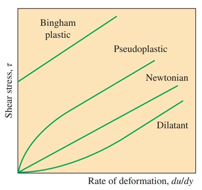
Figure 20- Variation of shear stress with the rate of deformation for Newtonian and non-Newtonian fluids (the slope of a curve at a point is the apparent viscosity of the fluid at that point).

Application Areas of Fluid Mechanics

On a broader scale, fluid mechanics plays a major part in the design and analysis of aircraft, boats, submarines, rockets, jet engines, wind turbines, biomedical devices, cooling systems for electronic components, and transportation systems for moving water, crude oil, and natural gas. It is also considered in the design of buildings, bridges, and even billboards to make sure that the structures can withstand wind loading. Numerous natural phenomena such as the rain cycle, weather patterns, and the rise of ground water to the tops of trees, winds, ocean waves, and currents in large water bodies are also governed by the principles of fluid mechanics.

Figure 21- Some application areas of fluid mechanics in everyday life.

Aerospace and Aeronautical Engineering

In aeronautics and aerospace engineering, fluid mechanics is essential for analyzing airflow around aircraft bodies. The shape and performance of airfoils, wings, and propulsion systems are directly influenced by fluid flow behavior. Engineers use fluid simulation software to conduct CFD fluid mechanics simulations that predict aerodynamic forces, reduce drag, and enhance fuel efficiency. The Navier-Stokes equations are fundamental in modeling airflow in these high-speed environments.

Figure 22- Bullet Aerodynamics CFD Simulation – 6DOF Dynamic Mesh: Application of CFD in Fluid Mechanics

Civil Engineering

Civil engineers apply fluid mechanics in engineering for tasks such as pumping concrete, managing water distribution systems, and designing HVAC systems in buildings. Wind-induced vibrations and noise are also studied using fluid mechanics formulas to ensure structural safety and comfort. CFD software helps simulate wind loads on tall structures and design energy-efficient ventilation systems.

Figure 23- Cross Ventilation of Building CFD Simulation, Numerical Paper Validation: Application of CFD in Fluid Mechanics

Biomedical Engineering

In biomedical engineering, fluid mechanics helps model the fluid flow of blood in arteries and veins. This is crucial for designing artificial heart valves, optimizing drug delivery systems, and studying fluid mechanics examples like micro-particle behavior. CFD simulations support doctors and researchers in analyzing complex biological flows and ensuring the effectiveness of medical devices

Figure 24- Blood Pulse Flow in Aneurysm CFD Simulation: Application of CFD in Fluid Mechanics

Marine Engineering

Fluid mechanics applications are vital in marine engineering for the design of ships, submarines, and offshore structures. CFD tools allow for the simulation of fluid dynamics in ocean environments, ensuring that vessels perform safely and efficiently under various sea conditions.

Figure 25- Underwater Glider Movement Using Dynamic Mesh CFD Simulation: Application of CFD in Fluid Mechanics

Mechanical Engineering

In mechanical engineering, components such as pumps, compressors, turbines, and heat exchangers rely heavily on fluid flow analysis. Engineers use fluid mechanics simulation software to improve the performance, safety, and efficiency of these devices. Whether designing a hydraulic system or analyzing a cooling system, CFD is essential in modern mechanical design processes.

Figure 26- Hydraulic Gear Pump CFD Simulation Using Dynamic Mesh: Application of CFD in Fluid Mechanics

Simulation of Fluid Mechanics by ANSYS Fluent

ANSYS Fluent is one of the most powerful and widely used fluid mechanics simulation software tools in the field of Computational Fluid Dynamics (CFD). Designed to simulate a broad range of fluid mechanics phenomena, ANSYS Fluent delivers high accuracy and flexibility for engineers and researchers. At its core, the software uses the finite volume method to solve the Navier-Stokes equations, enabling robust simulation of fluid flow, heat transfer, and chemical reactions. Fluent offers advanced CFD simulation methods for both laminar and turbulent flow regimes, including a variety of viscosity models and turbulence models such as k-ε, k-ω, and LES.

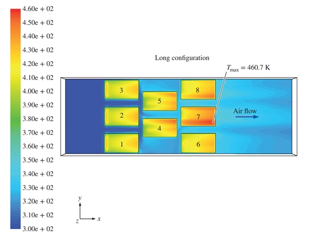
Figure 27- CFD results for the chip cooling example, long configuration: temperature contours as viewed from directly above the chip surfaces, with T values in K on the legend. The location of maximum surface temperature is indicated; it occurs near the end of chips 1, 2, and 3 are also seen, indicating high surface temperatures at those locations.

One of the key strengths of CFD in fluid mechanics with ANSYS Fluent is its ability to handle complex geometries and boundary conditions while allowing detailed customization of solver settings. Users can select from multiple pressure-velocity coupling schemes and numerical discretization methods based on the simulation requirements. ANSYS Fluent is ideal for simulating applications in aerospace, mechanical, civil, biomedical, and marine engineering. Its comprehensive tools enhance fluid flow modeling, support design validation, and contribute to the optimization of fluid-related systems across industries.

CFDLAND Expertise in Fluid Mechanics Modeling Using ANSYS Fluent

At CFDLAND, we specialize in fluid mechanics modeling through advanced CFD simulation using ANSYS Fluent. Our team of experts has extensive experience in simulating complex fluid dynamics phenomena. Whether you’re working on an academic research project or an industrial application, you can rely on CFDLAND’s CFD experts to deliver accurate, high-quality simulation results. We tailor every project to meet your specific needs, using validated methods and best practices in CFD analysis.

To request a custom CFD project, simply visit the ORDER PROJECT page and let us know your requirements. Explore our completed CFD simulation projects using ANSYS Fluent by visiting the CFD SHOP. Many of our top fluid mechanics simulations are also featured on this page — browse through and discover detailed case studies and training resources that might align perfectly with your goals.