An Airborne Wind Turbine (AWT) represents the future of green energy. Unlike traditional turbines fixed to the ground, an AWT flies at high altitudes where the wind is much stronger and more consistent. This allows it to generate significantly more power. However, designing these flying rotors is complex. Engineers must understand how the air flows around the blades while they are spinning high in the sky.

To solve this challenge, we use Airborne Wind Turbine CFD simulation. This method allows us to visualize the invisible wind forces on the computer. In this project, we perform a detailed Aerodynamic analysis of a horizontal axis AWT. We use ANSYS Fluent to model the airflow and calculate the forces that keep the turbine flying and generating electricity. For those interested in the fundamentals of flow physics, please explore our Fluid mechanics tutorials. Our study is based on the reference paper “Aerodynamic analysis of an airborne wind turbine…” by Saleem and Kim [1].

• Reference [1]: Saleem, Arslan, and Man-Hoe Kim. “Aerodynamic analysis of an airborne wind turbine with three different aerofoil-based buoyant shells using steady RANS simulations.” Energy Conversion and Management177 (2018): 233-248.

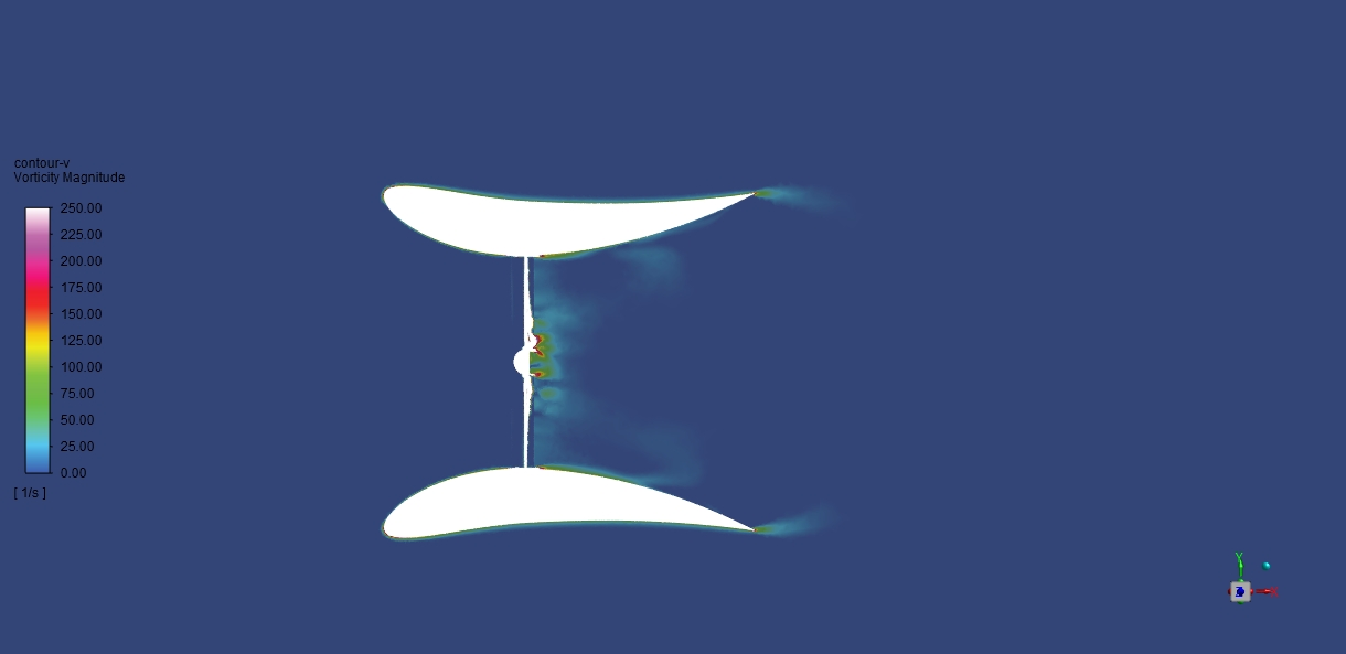
Figure 1: The profile of the wind turbine rotor used in this simulation [1].

Simulation Process: Modeling Rotation with MRF

Simulating a rotating machine like an Airborne Wind Turbine Using MRF Fluent requires a specific setup. First, we created the 3D geometry. We divided the domain into three distinct zones. There is a small rotating zone surrounding the blades, a large stationary zone for the far-field air, and a special third “control zone” behind the turbine. This control zone helps us refine the mesh exactly where the wake forms. The final mesh is extremely detailed, containing a total of 13,739,868 elements. This high number of cells ensures that our CFD simulation results are precise and independent of the grid size.

For the physics setup in ANSYS Fluent, we chose a steady-state approach. Since the wind hits the blades at a constant angle, we do not need to run a slow transient simulation. Instead, we used the MRF (Multi-Reference Frame) technique. This is the industry standard for MRF CFD studies. It allows us to freeze the rotor in position but simulate the physics of rotation by adding centrifugal and Coriolis forces to the equations. We set the rotation speed of the turbine to 190 rpm. This setup makes the calculation efficient while still capturing the complex aerodynamics of the rotor.

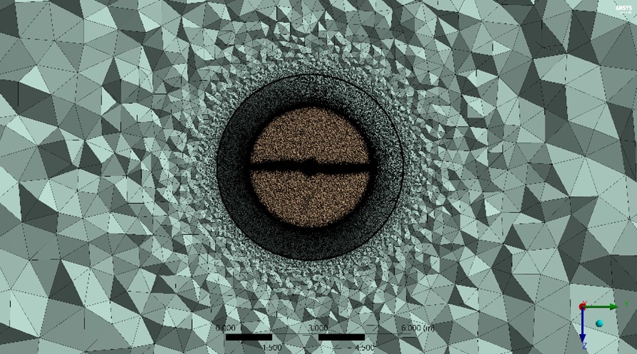
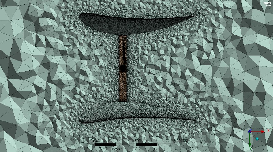
Figure 2: The high-quality computational mesh used for the Airborne Wind Turbine CFD analysis.

Post-processing: Wake Structure and Aerodynamic Loading

The results of the Airborne Wind Turbine CFD simulation provide a fascinating look into the aerodynamics of high-altitude power generation. Figure 3 displays the velocity streamlines, which act as a map of the wind’s speed and direction. As the wind approaches the turbine, it is forced to move around the spinning blades. We can clearly see regions of red and orange near the blade tips, indicating that the airflow has accelerated significantly. The simulation predicts a maximum velocity of 56.4 m/s in these regions. This acceleration is crucial because higher wind speed translates to higher kinetic energy extraction. Beyond the turbine, the streamlines show a long, twisting trail of blue and green. This is the wake region. The wake represents the energy that the turbine has removed from the wind. It is characterized by slower, swirling air that extends far downstream. Understanding the shape and length of this wake is vital for designing fleets of airborne turbines, as placing one turbine in the wake of another would drastically reduce its efficiency.

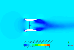
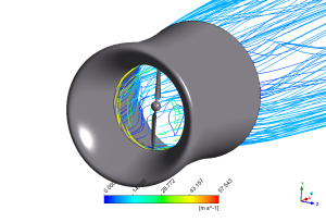
Figure 3: Velocity streamlines showing the flow acceleration and the large wake structure behind the turbine.

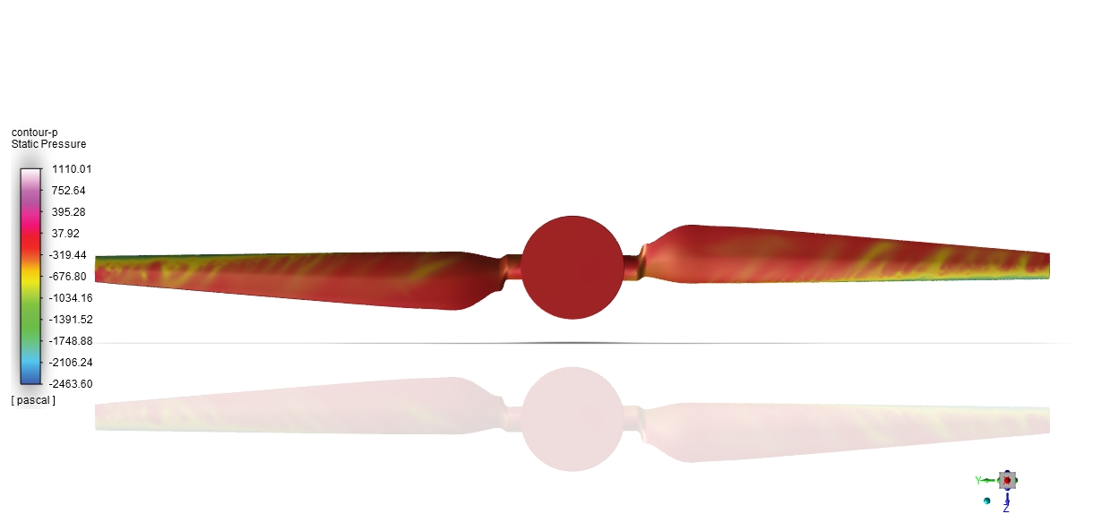
Figure 4 offers a deeper insight into the forces driving the turbine by showing the pressure contours on the blade surfaces. The physics of lift generation relies entirely on pressure differences. The contour plot reveals a stark contrast between the front and back of the blades. On the front surface, we see a red zone indicating high pressure, while on the back surface, there is a blue zone indicating low pressure. The simulation calculates this pressure difference to range from a minimum of -591 Pa to a maximum of 90.9 Pa. This specific gradient is what creates the aerodynamic force. The high pressure pushes against the blade while the low pressure pulls it forward. This combined force generates the torque that spins the rotor at 190 rpm. By accurately predicting these values, the Airborne Wind Turbine Fluent simulation proves that the blade design is effective at converting wind energy into mechanical rotation, even under the complex conditions of high-altitude flight.

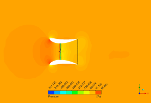
Figure 4: Pressure contours revealing the high and low-pressure zones on the blades that generate lift and torque.

Key Takeaways & FAQ

• Q: What is the advantage of an Airborne Wind Turbine (AWT)?
  • A: The main advantage is access to better wind. Winds at high altitudes (above 300 meters) are stronger and more steady than winds near the ground. An Airborne Wind Turbine CFD simulation helps engineers design rotors that can withstand these high speeds and generate more electricity than traditional ground-based turbines.
• Q: Why use the MRF method instead of a transient simulation?
  • A: The MRF (Multi-Reference Frame) method is a steady-state approximation. It is much faster than a full transient simulation. For a turbine spinning at a constant speed like 190 rpm, the flow field relative to the blade does not change much over time. MRF captures the rotation physics accurately without the high computational cost of time-stepping.
• Q: What does the pressure difference tell us?
  • A: The pressure difference is the source of power. The simulation showed a range from -591 Pa to 90.9 Pa. This difference between the high-pressure side and the low-pressure side creates the “Lift” force. This lift is what physically pushes the blade and makes the turbine rotate.