In the world of fluid dynamics, how a fluid interacts with a wall is very important. Usually, we assume that fluid molecules stick completely to the wall. This is called “non-slip flow.” However, in very small devices, like microchannels, this rule changes. The fluid molecules might slide or slip along the wall. This is called “slip flow.” This happens when the channel is so small that it is almost the same size as the distance molecules travel between collisions. Understanding this behavior is crucial for designing lab-on-a-chip devices and nanofluidic systems.

In this Microchannel Slip Flow CFD simulation, we explore these two different regimes. We aim to study the specific differences caused by slip and non-slip conditions inside a simple channel. We base our simulation setup on the concepts found in the research paper by Hosseini et al. (2014). However, instead of using standard settings, we face a challenge. ANSYS Fluent does not always have the built-in equations for this specific slip behavior. Therefore, we must use a custom code, known as a User-Defined Function (UDF), to define the physics correctly.

• Reference [1]: Hosseini, Seyed Mohammad Javad, Ataallah Soltani Goharrizi, and Bahador Abolpour. “Numerical study of aerosol particle deposition in simple and converging–diverging

Figure 1: Difference between slip and non-slip boundary conditions.

Simulation Process: Microchannel Geometry and UDF Slip Boundary Setup

For this ANSYS Fluent Microchannel simulation, we started by creating the computational domain. We used ANSYS Design Modeler to draw a simple 2D channel. Since we are looking at flow properties, a 2D representation is sufficient and saves calculation time. After the design was complete, we moved to the meshing stage. We generated a structured mesh grid. This is very important. We made the mesh much denser near the walls. We did this because the most interesting changes in velocity happen right at the boundary, and we need a fine grid to capture them.

The most critical part of this simulation is the physics setup in ANSYS Fluent. As mentioned before, the standard software assumes that the fluid speed at the wall is zero (non-slip). To simulate the slip regime, we could not use the default buttons. Instead, we wrote a User-Defined Function (UDF) in C language. This script tells the solver that the fluid velocity at the wall is not zero but depends on the shear stress and the properties of the gas. We compiled this UDF and applied it to the wall boundaries of the microchannel. This allows us to accurately model the molecular-level interactions that happen in microscale flows.

Post-processing: Velocity Profile Analysis of Slip vs Non-Slip Flow

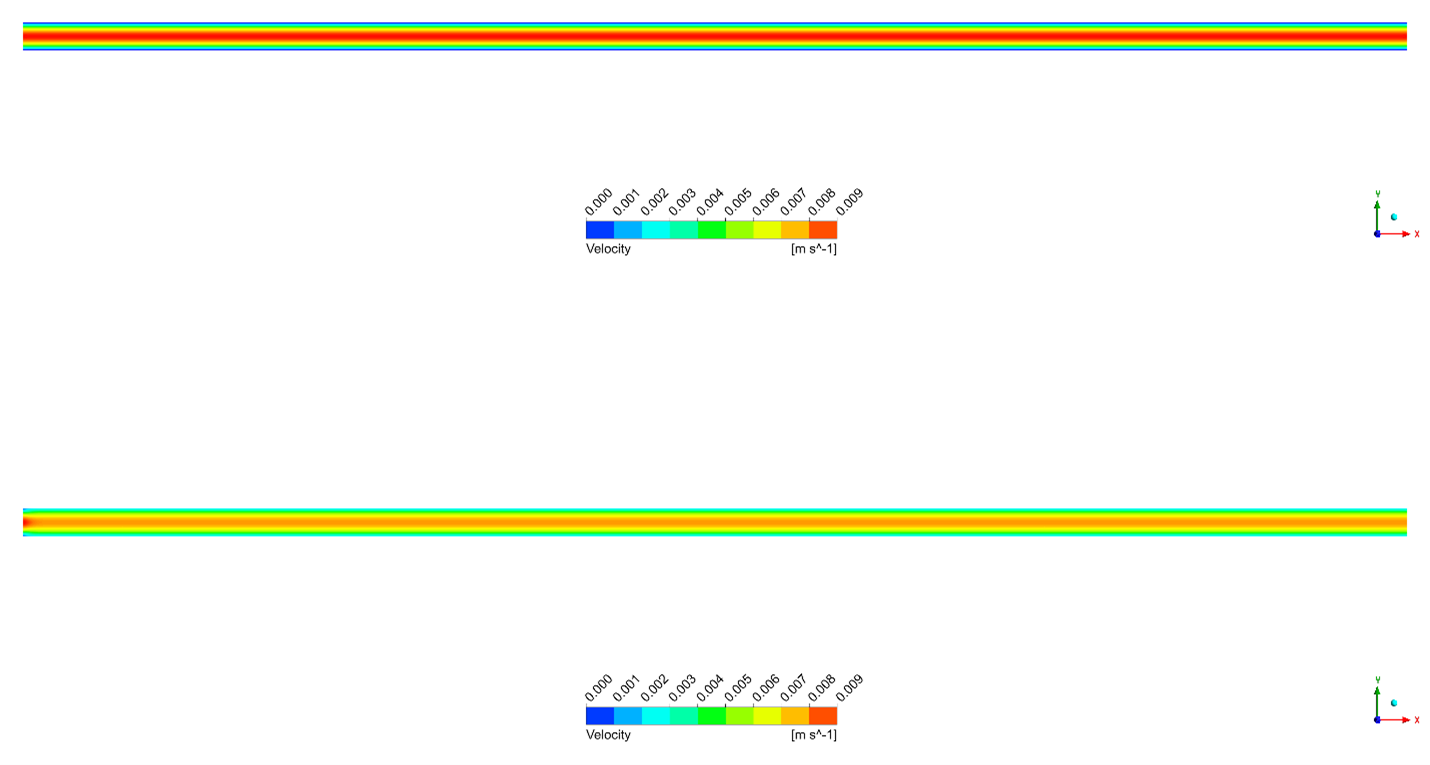
In this section, we analyze the results of our Microchannel CFD investigation. We compare the velocity contours and profiles of the two different flow regimes to understand their impact. First, let us look at the Velocity Contours (Figure 2). The visual difference is clear. In the non-slip scenario, we see the traditional pattern. The velocity is zero at the walls and reaches a high peak in the center. The dark red color in the center of the non-slip channel indicates a very high maximum velocity. On the other hand, the slip flow regime looks different. The velocity gradient near the wall is much lower. This means the change in speed from the wall to the center is not as sharp as in the non-slip case.

Figure 2: Velocity distribution along the microchannel: a) non-slip b) slip flow regime.

Second, we analyze the Sectional Velocity Profiles (Figure 3) to get exact numbers. The blue line represents the non-slip flow. It shows a perfect parabolic shape with a high peak. The red line represents the slip flow. Here, we can clearly see that the velocity at the wall is not zero. The fluid is actually moving along the boundary. Because the fluid is moving at the walls, it does not need to move as fast in the center to push the same amount of mass through. Consequently, the maximum centerline velocity for the slip case is approximately 15% to 20% lower than the non-slip case. The slip condition creates a flatter, more uniform velocity distribution across the width of the channel. This proves that the UDF successfully modified the boundary physics to mimic real microfluidic behavior.

Figure 3: Velocity profile on a section line – red (slip) and blue (non-slip).

Key Takeaways & FAQ

• Q: What is the main difference between Slip and Non-slip flow?
  • A: In non-slip flow, fluid velocity at the wall is zero; it sticks to the surface. In slip flow, the fluid velocity at the wall is not zero; it slides along the surface. This usually happens in very small (micro) channels.
• Q: Why is a User-Defined Function (UDF) needed here?
  • A: Standard CFD software typically uses the non-slip condition by default. To simulate the complex physics of molecules slipping at the wall in a microchannel, we need to add custom mathematical equations using a UDF.
• Q: How does slip flow affect the maximum velocity?
  • A: Because the fluid moves at the walls in slip flow, the flow is more spread out. This causes the maximum velocity in the center of the channel to be about 15-20% lower compared to non-slip flow.