UDF Macros in ANSYS Fluent | The Comprehensive Guide

In our previous blog post, we introduced the fundamentals of User Defined Functions (UDFs) in ANSYS Fluent. Now, we’ll explore deeper into one of the most important aspects of UDF development: DEFINE macros. These powerful tools are the building blocks that allow your custom code to communicate with the ANSYS Fluent solver at specific points during the simulation process.

UDF macros provide a structured interface to enhance Fluent’s capabilities, letting you implement custom boundary conditions, define specialized material properties, add source terms to equations, and much more. Understanding how to use these macros effectively is essential for creating efficient and powerful customizations in your CFD simulations.

As you’ll see in our UDF CFD Simulation Tutorials and examples throughout this guide, mastering these macros opens up endless possibilities for your CFD modeling. Whether you’re working on complex fluid flows, heat transfer problems, or multiphase simulations, UDFs can help you implement physics that aren’t available in the standard ANSYS Fluent package.

In this comprehensive guide, we’ll explore the various categories of UDF macros, explain their syntax and implementation, and provide practical examples to help you master these tools for your ANSYS Fluent simulations.

Understanding DEFINE Macros in ANSYS Fluent: The Basics

In ANSYS Fluent, DEFINE macros are the building blocks of UDF programming. Each macro has a similar structure but is used for a different task in the simulation process. Think of these macros as special entry points that tell Fluent when and how to run your custom code.

When you write a UDF, you’re creating instructions that will execute at specific times during the simulation. For example, some macros run at the beginning of each iteration, while others might only execute when initializing the solution or when applying boundary conditions.

How DEFINE Macros Work

All UDF macros follow this pattern:

DEFINE_MACRO_TYPE(name, parameters…)

{

    // Your custom C code here

}

Here’s what each part means:

• DEFINE_MACRO_TYPE: The type of macro you’re using (like DEFINE_PROFILE)
• name: What you want to call your function
• parameters: Information that Fluent gives to your macro

Every UDF file must start with:

#include “udf.h”

This header connects your code to Fluent’s internal data structures, functions, and macros. Without this line, your UDF won’t compile correctly because it won’t recognize any of the ANSYS Fluent-specific functions and macros you need to use.

Types of UDF Macros in ANSYS Fluent

ANSYS Fluent has plenty of UDF macros that are grouped into various categories based on what they do. Knowing about these groups will help you pick the best macro for your needs. Let’s look at each category in detail so you can understand when and why you might use these different types of macros in your CFD simulations.

1. General Purpose DEFINE Macros

These macros perform general functions independent of specific physics models. They’re often used to control the simulation process or monitor results during calculation.

Macro	What It Does	When It Works
DEFINE_ADJUST	Changes values before solving	At the start of each step
DEFINE_INIT	Sets starting conditions	When you initialize
DEFINE_EXECUTE_AT_END	Runs code after solving	At the end of each step
DEFINE_ON_DEMAND	Runs when you ask for it	When clicked in the menu
DEFINE_DELTAT	Controls time step size	During time-dependent simulations
DEFINE_RW_FILE	Reads/writes files	When loading/saving

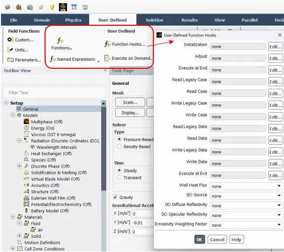
Figure 1: UDF Hooks in ANSYS Fluent

For example, you might use DEFINE_ADJUST to calculate a volume-averaged temperature at the start of each iteration, or DEFINE_INIT to create a complex initial temperature distribution that isn’t possible with Fluent’s standard initialization tools.

These macros give you control over the simulation process itself, allowing you to monitor results, adjust parameters on the fly, or implement advanced solution control techniques.

2. Model-Specific DEFINE Macros

These macros are designed for interacting with specific physics models. They let you customize the behavior of particular aspects of your CFD simulation.

Macro	What It Does	Where To Use It
DEFINE_PROFILE	Sets custom boundary conditions	Inlets, walls, etc.
DEFINE_PROPERTY	Changes material properties	Fluids, solids
DEFINE_SOURCE	Adds extra terms to equations	Energy sources, forces
DEFINE_DIFFUSIVITY	Changes how things spread	Species mixing, heat transfer
DEFINE_PRANDTL	Affects turbulence models	Turbulent flows
DEFINE_VR_RATE	Sets reaction speeds	Chemical reactions

These macros are particularly useful when you need to implement physics that aren’t available in standard models. For instance, you might use DEFINE_PROPERTY to create a complex non-Newtonian viscosity model that depends on both temperature and shear rate, or use DEFINE_SOURCE to add a chemical reaction heat source that depends on local species concentrations.

By using these model-specific macros, you can significantly extend ANSYS Fluent’s modeling capabilities to handle specialized physics for your specific engineering application.

3. Multi-Phase DEFINE Macros

For simulations involving multiple phases, these specialized macros allow you to control how different phases interact with each other:

Macro	What It Does
DEFINE_MASS_TRANSFER	Controls mass moving between phases
DEFINE_EXCHANGE_PROPERTY	Sets how phases interact
DEFINE_CAVITATION_RATE	Controls bubble formation
DEFINE_VECTOR_EXCHANGE_PROPERTY	Sets directional properties between phases

Multi-phase flows are among the most complex phenomena to model in CFD simulations. These macros give you fine control over phase interactions. For example, you might use DEFINE_MASS_TRANSFER to model condensation or evaporation processes with custom physics, or DEFINE_CAVITATION_RATE to implement specialized bubble formation models for pump simulations.

If you’re working on problems like evaporation, condensation, boiling, or other multi-phase phenomena, these macros allow you to implement physics beyond what’s available in the standard ANSYS Fluent models.

4. Particle Tracking DEFINE Macros

For particle tracking and discrete phase modeling, these macros help you control how particles behave in your simulation:

Macro	What It Does
DEFINE_DPM_INJECTION	Controls where particles start
DEFINE_DPM_BODY_FORCE	Adds forces to particles
DEFINE_DPM_DRAG	Changes how fluid pulls on particles

The Discrete Phase Model (DPM) in ANSYS Fluent is used to track particles, droplets, or bubbles within a continuous fluid. These macros let you customize particle behavior. For instance, you might use DEFINE_DPM_INJECTION to create a time-varying spray pattern in a fuel injector simulation, or DEFINE_DPM_BODY_FORCE to add electromagnetic forces on charged particles.

These macros are essential for accurately modeling sprays, particle-laden flows, and other discrete phase phenomena in your CFD simulations.

5. Moving Mesh DEFINE Macros

For simulations with moving or deforming meshes, these macros control how your mesh changes during the simulation:

Macro	What It Does
DEFINE_GRID_MOTION	Controls how mesh moves
DEFINE_CG_MOTION	Controls object motion
DEFINE_GEOM	Creates shape definitions

Dynamic mesh simulations are used for problems where boundaries move or deform, such as valve operations, piston movement, or fluid-structure interaction. These macros give you precise control over how the mesh moves. For example, you might use DEFINE_GRID_MOTION to implement a custom valve-lifting profile, or DEFINE_CG_MOTION to model the six-degree-of-freedom motion of a floating object.

If your CFD simulation involves any kind of moving parts or boundaries, these macros will be essential tools in your UDF development process.

6. Custom Equations DEFINE Macros

For adding and solving custom transport equations beyond what’s built into ANSYS Fluent, these macros are invaluable:

Macro	What It Does
DEFINE_UDS_FLUX	Sets how your variable moves
DEFINE_UDS_UNSTEADY	Handles time changes
DEFINE_UDS_BOUNDARY	Sets edge conditions

User-Defined Scalars allow you to solve additional transport equations for quantities not included in standard ANSYS Fluent models. For example, you might need to track the concentration of a pollutant, the age of fluid, or some other custom parameter. These macros let you control every aspect of how these custom equations are solved.

If you’re working with specialized physics that require tracking additional variables beyond what’s built into Fluent, these macros will be essential for your UDF development.

Most Important UDF Macros with Examples

Now let’s examine the most commonly used UDF macros with practical examples. Understanding these key macros will give you the foundation you need to create effective UDFs for almost any CFD simulation challenge.

DEFINE_PROFILE: Custom Boundary Conditions

The DEFINE_PROFILE macro lets you create position-dependent or time-dependent boundary conditions. This is one of the most frequently used macros because it allows you to implement realistic boundary conditions that change with time, position, or other parameters.

How to write it:

DEFINE_PROFILE(name, thread, position)

What each part means:

• name: Your function name – this is how you’ll identify your UDF in the Fluent interface
• thread: Boundary thread where profile will be applied – this is a pointer to the boundary zone data structure
• position: Index identifying which boundary value to set – this tells Fluent which variable you’re modifying (velocity, temperature, etc.)

Example: Non-uniform velocity profile (Atmospheric Boundary Layer (DEFINE_PROFILE))

When simulating environmental flows or wind engineering problems, accurately modeling the atmospheric boundary layer (ABL) is crucial. Here’s how you can implement a realistic ABL velocity profile using the DEFINE_PROFILE macro.

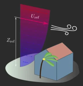
Figure 2: Instantaneous velocity profile for modeling atmospheric airflow

This UDF implements the standard logarithmic wind profile based on Monin-Obukhov similarity theory, which is widely used in meteorology and wind engineering. The key relations for velocity profile, kinetic energy and dissipation rate include:

The resulting velocity profile increases logarithmically with height, accurately reflecting how wind behaves in the lower atmosphere due to surface friction and turbulence. As a result, you`ll be able to apply these non-uniform parameters in the boundary condition panel:

Figure 3: Wind profile velocity UDF applied on inlet boundary

This macro of UDF is perfect for simulating pulsating flows, like blood flow in arteries or time-varying inlet conditions in an engine. You can also create position-dependent profiles, for example, to implement a parabolic velocity profile that varies across the boundary.

How to use this UDF:

1. Save and compile the UDF (Define → User-Defined → Functions → Compile)
2. Go to your inlet settings
3. For velocity, pick “UDF”
4. Choose your UDF from the list

DEFINE_PROPERTY: Custom Material Properties

The DEFINE_PROPERTY macro allows you to define custom material properties that can vary with temperature, position, or other parameters. This is extremely useful when you need to model materials with complex behavior that can’t be represented by constant values or built-in functions.

How to write it:

DEFINE_PROPERTY(name, cell, thread)

What each part means:

• name: Your function name
• cell: Which cell we’re looking at
• thread: Which zone the cell is in

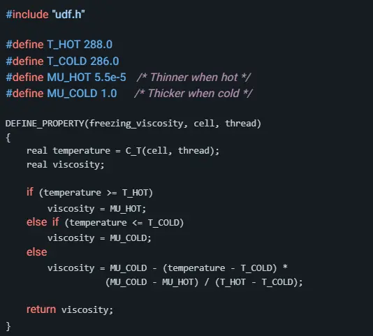
Example: Temperature-Changing Viscosity

This UDF creates a temperature-dependent viscosity model that simulates solidification by increasing viscosity at lower temperatures. In this code:

• C_T(cell, thread) retrieves the temperature for the current cell
• The if-else structure creates a piecewise function where viscosity:
  • Is low (liquid-like) above the hot temperature
  • Is high (solid-like) below the cold temperature
  • Varies linearly between these temperatures

This type of UDF is essential for simulating materials with phase change, non-Newtonian fluids, or any situation where material properties change based on local conditions. For example, you might use this approach to model honey or oil that gets thicker in cold regions, or to handle the complex viscosity behavior of polymers.

How to use this UDF:

1. Save and compile the UDF
2. Go to Define → Materials
3. For viscosity, pick “user-defined”
4. Choose your UDF from the list

Once applied, ANSYS Fluent will call your UDF to calculate the appropriate viscosity in each cell based on the local temperature. This gives you a much more realistic simulation than using a constant viscosity value would provide.

DEFINE_SOURCE: Adding Extra Terms

The DEFINE_SOURCE macro allows you to add custom source terms to any of the transport equations being solved. This is extremely powerful because it lets you model phenomena that aren’t included in ANSYS Fluent’s standard physics models.

How to write it:

DEFINE_SOURCE(name, cell, thread, dS, eqn)

What each part means:

• name: Your function name
• cell: Which cell we’re looking at
• thread: Which zone the cell is in
• dS: Helper value for solving
• eqn: Which equation to change

Example: Magnetic Field Effects on Ferrofluid Flow

One powerful application of the DEFINE_SOURCE macro is modeling magnetic field effects in computational fluid dynamics. Consider this advanced example where we simulate an alternating non-uniform magnetic field affecting ferrofluid flow and heat transfer in a channel:

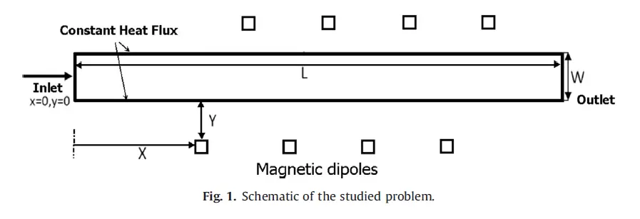
Figure 4: Non-uniform magnetic field applied by magnetic dipoles around the model

The UDF implements a model for the magnetic body force in the x-direction based on Rosensweig’s ferrohydrodynamic theory. The source term adds the effects of eight magnetic dipoles placed along the channel boundaries. In this implementation:

• The magnetic field at each point is calculated based on the superposition of fields from eight line dipoles
• Field gradients create forces on the magnetic fluid
• The resulting source term represents the momentum contribution from magnetic forces

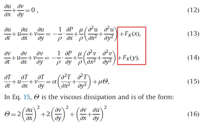
Figure 5: The magnetic field force added as source terms via UDF

To complete this model, you would need additional helper functions for calculating the magnetic field and its gradients, plus a similar source term for the y-direction. The results are depicted in the following figure:

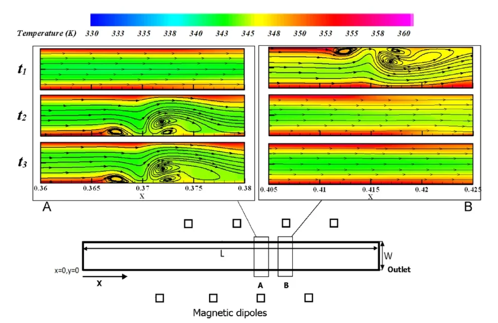
Figure 6: The flow pattern in the presence of magnetic field

This type of simulation is critical for studying magnetic cooling systems, targeted drug delivery, magnetic separation processes, and other emerging technologies that leverage magnetically responsive fluids.

How to use this UDF:

1. Save and compile the UDF
2. Go to Define → Cell Zone Conditions
3. Pick the zone for your heat source
4. Turn on source terms and pick energy equation
5. Set source to “user-defined”
6. Choose your UDF from the list

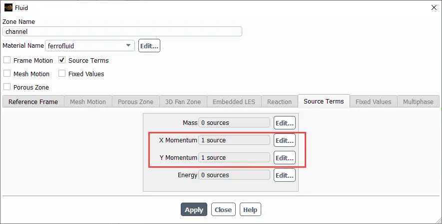
Figure 7: The source terms added in cell zone condition panel

DEFINE_INIT: Custom Starting Conditions

The DEFINE_INIT macro allows you to set custom initial conditions. This is particularly useful when you need a complex starting point for your simulation that can’t be achieved with ANSYS Fluent’s standard initialization options.

How to write it:

DEFINE_INIT(name, domain)

What each part means:

• name: Your function name
• domain: All the cells in your simulation

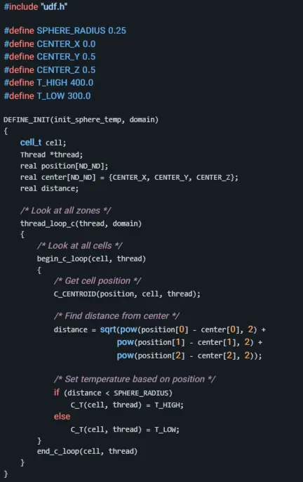
Example: Starting With A Hot Sphere

This UDF initializes the temperature field with a hot sphere surrounded by cooler fluid. In this code:

• thread_loop_c cycles through all cell zones (threads) in the domain
• begin_c_loop and end_c_loop create a loop through all cells in each zone
• C_CENTROID gets the position of each cell center
• Based on the distance from a defined center point, the cell’s temperature is set to either a high or low value

This type of initialization is perfect for setting up thermal stratification, initial temperature distributions for heat transfer studies, or any situation where you need a non-uniform starting point for your simulation. Without a UDF, creating such complex initial conditions would be nearly impossible.

How to use this UDF:

1. Save and compile the UDF
2. Go to Define → User-Defined → Function Hooks
3. Under “Initialization,” pick your UDF
4. Initialize your simulation with Solve → Initialize → Initialize

DEFINE_ADJUST: Making Calculations While Running

The DEFINE_ADJUST macro enables you to perform calculations at the beginning of each iteration. This is particularly useful for monitoring solution progress, updating variables, or implementing adaptive solution controls.

How to write it:

DEFINE_ADJUST(name, domain)

What each part means:

• name: Your function name
• domain: All the cells in your simulation

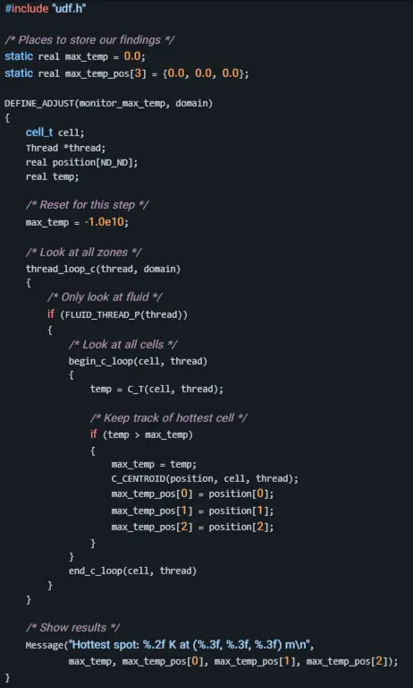
Example: Calculate Maximum Temperature

This UDF tracks the maximum temperature in the domain and reports it during each iteration. In this code:

• Static variables store the maximum temperature and its location between function calls
• FLUID_THREAD_P checks if the current thread is a fluid zone
• The code loops through all cells, comparing each cell’s temperature to the current maximum
• Message() prints the results to the console

This kind of monitoring is extremely useful for tracking critical parameters during your simulation without having to stop and check manually. You could use a similar approach to calculate average values, monitor convergence, or implement adaptive solution controls based on solution behavior.

How to use this UDF:

1. Save and compile the UDF
2. Go to Define → User-Defined → Function Hooks
3. Under “Adjust,” pick your UDF

After activating this UDF, it will run at the beginning of each iteration, printing the maximum temperature value and location to the console. This provides real-time monitoring of this important parameter throughout your simulation.

DEFINE_DELTAT: Controlling Time Steps

The DEFINE_DELTAT macro allows you to control the time step size in transient simulations. This gives you the power to adapt the time step based on flow conditions, leading to more accurate and efficient simulations.

How to write it:

DEFINE_DELTAT(name, domain)

What each part means:

• name: Your function name
• domain: All the cells in your simulation

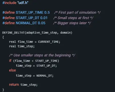
Example: Adaptive Time Step Based on Simulation Time

This UDF implements a simple adaptive time step strategy with smaller steps during the initial startup period. In this code:

• CURRENT_TIME gets the current simulation time
• A smaller time step is used during an initial “start-up” period
• A larger time step is used once the simulation has stabilized

Adaptive time stepping is crucial for efficient transient simulations. You could expand this approach to adjust the time step based on maximum velocity, gradients, or other solution-dependent variables. This ensures you use small time steps only when needed for accuracy, and larger time steps when possible for efficiency.

How to use this UDF:

1. Save and compile the UDF
2. Go to Solve → Run Calculation
3. Set “Time Step Size” to “User-Defined”
4. Pick your UDF from the list

With this UDF activated, your simulation will automatically adjust its time step size according to your custom logic, making it both more accurate during critical periods and more efficient during stable periods.

DEFINE_SR_RATE: Custom Surface Reaction Rates

For simulations involving chemical reactions on surfaces, the DEFINE_SR_RATE macro allows you to implement custom reaction rate models beyond what’s available in ANSYS Fluent’s standard surface chemistry options.

DEFINE_SR_RATE(name, f, t, r, mw, yi, rr)

• name: Your function name
• f: Face index
• t: Thread containing the face
• r: Reaction index
• mw: Array of molecular weights
• yi: Array of species mass fractions
• rr: Pointer to store the reaction rate

Example: Photocatalytic Degradation of Formaldehyde

We need a UDF that implements a modified Langmuir-Hinshelwood kinetic model for the photocatalytic degradation of formaldehyde on a TiO₂ catalyst surface. The reaction rate depends on:

• Local formaldehyde concentration
• Surface temperature
• UV light intensity, which varies throughout the reactor

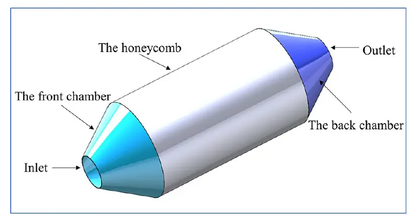
Figure 8: PHOTOCATALYTIC REACTOR VISUALIZATION

This type of model is essential for designing efficient honeycomb photocatalytic reactors for indoor air purification, as it accounts for:

• Adsorption-desorption equilibrium on the catalyst surface
• Temperature-dependent reaction kinetics
• Light intensity effects on photocatalytic activity

After compiling the UDF into ANSYS Fluent, it will be reachable from UDF Hooks section:

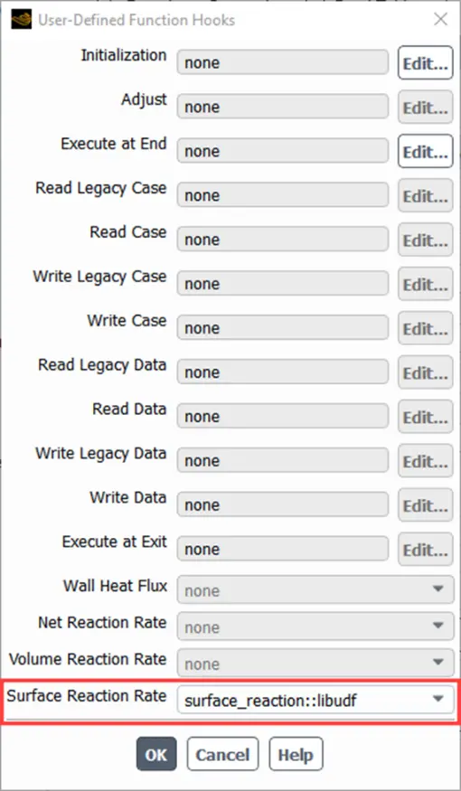
Figure 9: Surface reaction rate UDF in UDF Hooks of Fluent

Additional Macros for UDF Development

In addition to the DEFINE macros, ANSYS Fluent provides many supporting macros that help you access and manipulate data within your UDFs. These supporting macros are essential tools that work alongside the DEFINE macros to give you complete control over your CFD simulation.

Loop Tools

Loop macros allow you to iterate through mesh elements efficiently. Without these, accessing all cells or faces in your domain would be much more complex.

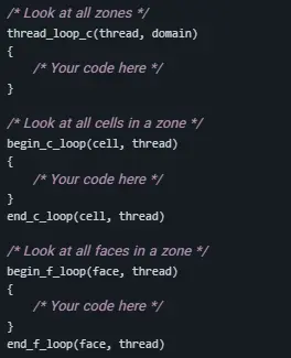
These macros make it easy to process every cell or face in your mesh. For example, you might use them to calculate average values across a zone, find maximum or minimum values, or apply custom operations to specific regions based on position or other criteria.

The loop macros handle all the complexities of mesh traversal, including parallel processing considerations, making your UDF code much cleaner and more efficient than manual looping would be.

Geometry Tools

Geometry macros provide access to spatial information about your mesh elements:

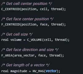
These macros let you access geometric properties like cell centers, volumes, face areas, and more. This information is often crucial for creating position-dependent behavior in your UDFs. For example, you might use cell positions to create spatially varying source terms, or face areas to calculate fluxes across boundaries.

Understanding these geometry macros is essential for creating UDFs that interact with the physical domain of your simulation.

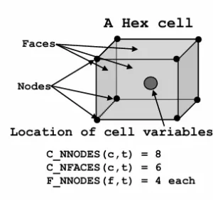
Figure 10: Structure of a hex element

Value Tools

Field variable macros allow you to access solution data at specific locations in your mesh:

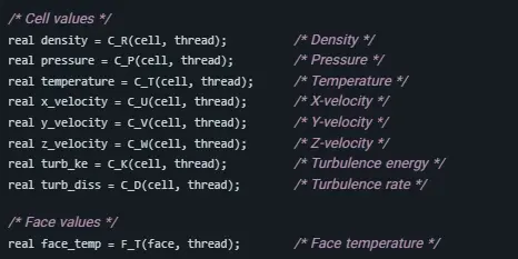
These macros give you direct access to the solution variables in each cell or face. This is critical for creating UDFs that respond to flow conditions. For example, you might need to access temperature to create temperature-dependent properties, or velocity components to calculate custom forces.

The field variable macros make it easy to retrieve these values without having to understand the complex data structures used internally by ANSYS Fluent.

How to Use UDF Macros in Your Simulations

To implement UDF macros in your ANSYS Fluent simulations, follow these steps. Even if you have never written a UDF before, these clear instructions will help you create, compile, and activate your first UDF.

Step 1: Write Your UDF Code

Create a text file with the .c extension containing your UDF code. You can use any text editor for this, such as Notepad, Notepad++, or Visual Studio. Start with the header file and define your functions using the appropriate DEFINE macros.

Step 2: Load Your UDF Into Fluent

In ANSYS Fluent:

1. Go to Define → User-Defined → Functions
2. Pick “Interpret” (for simple UDFs) or “Compile” (for complex UDFs)
3. Find your UDF file and click OK

Step 3: Use Your UDF

How you use your UDF depends on what kind it is:

• For boundary conditions (DEFINE_PROFILE):
  • Go to the boundary settings
  • For the value you want to change, pick “UDF”
  • Choose your UDF from the list
• For material properties (DEFINE_PROPERTY):
  • Go to Define → Materials
  • For the property you want to change, pick “user-defined”
  • Choose your UDF from the list
• For source terms (DEFINE_SOURCE):
  • Go to Define → Cell Zone Conditions
  • Turn on source terms for the equation you want
  • Set the source to “user-defined”
  • Choose your UDF from the list
• For other functions (DEFINE_INIT, DEFINE_ADJUST, etc.):
  • Go to Define → User-Defined → Function Hooks
  • Find the right section and pick your UDF

Conclusion

UDF macros are powerful tools that let you do more with ANSYS Fluent by adding custom features to your simulations. By learning about the different types of macros and how to use them, you can solve complex engineering problems that the standard features can’t handle.

In this guide, we’ve shown you the most important UDF macros in ANSYS Fluent – from changing boundary conditions and material properties to adding source terms and setting starting conditions. We’ve also shown you helper tools that make UDF writing easier.

By using these macros, you can create unlimited possibilities for your CFD simulations, adding custom physics, special boundary conditions, and unique analysis tools.

In our next blog posts, we’ll look at specific uses of UDF programming in ANSYS Fluent with complete examples for common engineering problems.

For hands-on practice with these techniques, check out our UDF CFD tutorials section where we show you step-by-step how to implement these examples.