What is a Courant Number? (CFL Number)

Kiarash Kord

The Courant number (CFL number) is a fundamental concept in computational fluid dynamics (CFD) that provides a stability condition and ensures the correct propagation of information within the computational domain. This article explores the Courant number meaning, the CFL condition, its derivation, and its practical consequences in CFD. The process of calculating the Courant number, its impact on stability, and methods for handling convergence issues when the CFL condition is violated will be discussed. Applications of the Courant number in various CFD solvers, including ANSYS Fluent and OpenFOAM, along with its role in HEC-RAS, are also examined. The article concludes with practical considerations for setting up simulations effectively.

Contents

What is the Courant Number?

The Courant number, also referred to as the CFL number (Courant-Friedrichs-Lewy number), is a dimensionless parameter that plays a crucial role in numerical simulations, particularly in CFD and other time-dependent problems. It determines the stability of numerical schemes, especially explicit time-marching methods. Mathematically, the Courant number formula (in 1D case) is given by:

$C = \frac{v \cdot \Delta t}{\Delta x}$

where:

C = Courant number

𝑣 = Velocity of the fluid or wave speed

Δ𝑡 = Time step size

Δ𝑥 = Spatial grid resolution

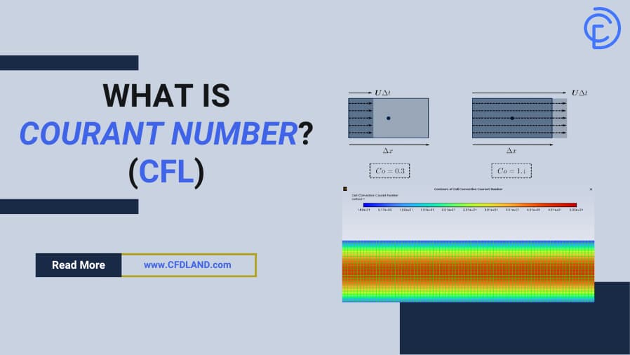
The Courant number meaning is straightforward: Over a time step Δ𝑡, the flow moves a distance UΔ𝑡 across the cell (Fig.1). The Courant number is the ratio of these two lengths or the fraction of the cell that moves across in a given time step. Hence it is a dimensionless quantity.

$C = \frac{\text{``Fluid Distance''}}{\text{``Cell Distance''}} = \frac{U \cdot \Delta t}{\Delta x}$

Fluid Distance = 𝑈⋅Δ𝑡 (the distance a fluid particle travels during one time step)

Cell Distance = Δ𝑥 (the size of a computational grid cell)

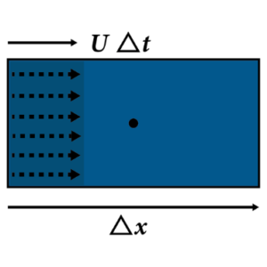
Figure 1- The Courant number conception

Explicit and Implicit Methods: Understanding Their Applications in Numerical Simulations

In numerical simulations, explicit and implicit methods are used to solve differential equations: Ordinary Differential Equations (ODEs) and Partial Differential Equations (PDEs). These methods provide approximate solutions when analytical solutions are not feasible. The choice between these methods depends on the nature of the problem, the required accuracy, and the available computational resources. It can also significantly influence the stability, accuracy, and efficiency of the solution process. Therefore, understanding the trade-offs between explicit and implicit methods is crucial for selecting the right approach for a given simulation.

Explicit Methods

In explicit methods, the solution at a given time step is explicitly calculated based on the known values from the previous time step. The governing equations are solved directly, with no need for solving large systems of equations. For a time-dependent PDE, the explicit method can be written as:

$u_{n+1} = u_n + \Delta t \cdot f(u_n,x)$

Un+1= Solution at the next time step
Un= Solution at the current time step
Δ𝑡= Time step size
f(Un,x)= Function representing the spatial derivatives and source terms

Implicit Methods

In implicit methods, the solution at a given time step depends on both the current and future time step values. This requires solving a system of linear or nonlinear equations at every time step, making the method more computationally intensive. For a time-dependent PDE, the implicit method can be written as:

$u_{n+1} = u_n + \Delta t \cdot f(u_{n+1},x)$

Un+1= Solution at the next time step (unknown and needs to be solved for)
Un= Solution at the current time step
Δ𝑡= Time step size
f(Un,x)= Function representing the spatial derivatives and source terms at the next time step

Table 1 shows a brief comparison between the Explicit and Implicit Methods.

Table 1- Comparison of Explicit and Implicit methods in numerical simulations

Feature	Explicit Methods	Implicit Methods
Stability	Conditioned by CFL (C≤1)	Often unconditionally stable
Time Step Size	Small time steps required for stability	Larger time steps allowed
Computational Cost	Lower (no systems to solve)	Higher (requires solving systems)
Implementation	Easier to implement	More complex to implement
Applicability	Suitable for problems with small time steps	Suitable for stiff problems or large time steps

Appropriate CFL Condition

If we want to discuss the requirements for convergence, we can say that, from a numerical perspective, time discretization can generally be classified into three methods: explicit, implicit, and semi-implicit. In general, for simulation convergence, it is preferable to keep the Courant number around one. This condition, known as the CFL condition, is particularly crucial when using explicit methods. The main challenge in maintaining the CFL condition is that it leads to longer and more computationally expensive CFD simulations.

Semi-implicit and implicit methods help relax these strict CFL constraints, allowing for larger time steps and Courant numbers greater than one. However, in implicit methods, the Courant number should not be excessively large, as it may lead to inaccurate results. Since the Courant number depends on both the mesh size and time step, mesh quality also plays a crucial role. For instance, very small cells or high aspect ratio cells can increase errors or cause divergence when using large time steps.

Courant number example

As mentioned, the Courant Number expresses that the distance information travels during a time step within the mesh must be lower than the distance between mesh elements (Fig.2). In other words, information (Temperature, Pressure, Velocity, etc.) from a given cell or mesh element must have enough time to propagate only to its immediate neighbors to maintain numerical stability.

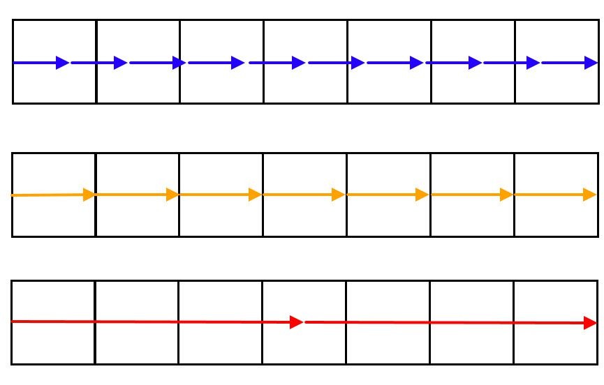
Figure 2- visual representation of Courant numbers equal to 0.7 (blue), 1 (orange), and 3.5 (red). Keep Courant number below 1.

The Fig.3 illustrates the Courant number (Co) condition in numerical simulations, comparing two cases (Co = 0.3 and Co = 1.1) to show how the choice of time step (Δt) and spatial discretization (Δx) affects numerical stability.

Figure 3- Effect of Courant number on flow propagation

Understanding the Two Cases:

Left Image (Co = 0.3)

The flow moves 30% of a cell size (Δx) during one time step (UΔt).
This results in a stable condition for explicit time integration methods, ensuring accurate simulation results.

Right Image (Co = 1.1)

The flow moves more than a full cell (110%) within a time step.
This violates the CFL condition for explicit methods, potentially causing numerical instability, oscillations, or divergence.

The Two and General n-Dimensional Case

In the two-dimensional case, the CFL condition becomes:

$C = \frac{u_x\Delta t}{\Delta x} + \frac{u_y\Delta t}{\Delta y} \leq C_{\text{max}}$

By analogy, for the general n-dimensional case, the CFL condition is:

$C = \Delta t \sum_{i=1}^n \frac{u_{x_i}}{\Delta h_i} \leq C_{max}$

Effect of Numerical Methods on Cmax

The value of Cmax depends on the numerical method used:

For explicit (time-marching) solvers, typically Cmax=1 is required for stability.
Implicit (matrix-based) solvers are less sensitive to numerical instability, allowing for larger values of Cmax .

The Courant number in an arbitrary 3D cell

As we know, calculating the Courant number and its physical meaning for 1D cells is simple. However, CFD simulation software such as OpenFOAM, ANSYS Fluent and HEC-RAS supports a wide range of cell shapes, including hexahedra, wedges, prisms, pyramids, tetrahedra, tetrahedral wedges, and polyhedral (Fig.4). Additionally, these cells are often not perfectly shaped. This raises the question of how to calculate the Courant number for an arbitrary element that may have slight imperfections in its geometry.

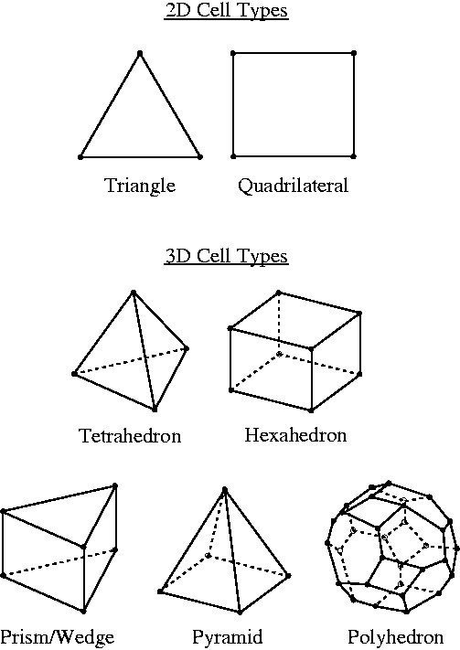
Figure 4- Read more about Cell Types

Calculating Δx for an arbitrary 3D cell

Calculating Δx for an arbitrary 3D cell is a critical challenge in accurately determining the Courant number (Fig.5). The irregular shape of the cell requires using geometric properties (volume and surface area) to approximate Δx.

Figure 5- Determining the Characteristic Length (Δx) for an Arbitrary 3D Cell

In fact, the spatial step size, Δx, is not straightforward to determine for irregular 3D cells. A common approach is to calculate Δx using the formula:

$\Delta x = \frac{\text{Cell Volume (V)}}{\text{Total Surface Area (A)}} \text{ or } \Delta x = \frac{V}{A}$

This formula relates the cell’s volume (V) to its surface area (A), providing an estimate of the “average” distance that information travels across the cell. The total surface area is simply equal to the sum of each face area that closes the volume (Fig.6).

$A = A_1 + A_2 + A_3 + …A_N$

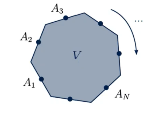
Figure 6- Surface Area and Volume Representation of an Arbitrary 3D Cell

The velocity normal for an arbitrary 3D cell

To determine the Courant number, we also require the velocity component normal to each face of the cell (Fig.7). This can be obtained by computing the dot product of the face velocity vector Uf and the unit normal vector n, which points toward the cell centroid: Uf.n

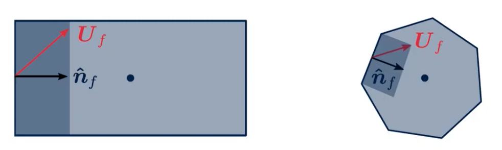
Figure 7- Velocity normal to the face

At this point, it is important to note that if we calculate the velocity normal to each face and sum these values, the result will be zero due to the continuity equation. This occurs because the net mass flow into and out of each cell must balance to zero. To address this, instead of summing the normal velocity components directly, we sum the magnitudes of Uf.n for each face. This effectively reverses half of the flux, ensuring the total is not zero. However, to obtain the true flux, we must take only half of this sum. Taking this adjustment into account, we arrive at the final expression for the Courant number:

$C = \frac{1}{2}\Delta t\sum \frac{|Uf \cdot \vec{n}|A}{V}$

where,

Uf: Velocity at that face
V: Volume of the cell
A: Area of the face
n: Normal vector to face
Sigma: Represents sum along all faces.

Here, 1/2 considered, we are reversing direction of half of flux, as mod || considered.

The courant number field

In reality, every cell in the mesh has a different Courant Number and hence it is a field that can be plotted like any other variable. The Courant number field shown in the Fig. 8 represents the spatial distribution of the Courant number across a computational domain, where the Courant number is a dimensionless parameter that governs the stability of explicit numerical schemes in fluid dynamics simulations. Higher Courant number regions (red/orange) indicate areas with faster fluid velocities, smaller grid cells, or both, while lower Courant number regions (blue) correspond to slower velocities or coarser grid resolution. The Courant number is calculated using local flow velocity, time step size, and grid spacing, and it must typically remain below 1 for explicit solvers to ensure numerical stability. This visualization helps identify regions that may require adjustments to the grid or time step to maintain stable simulations. CFD solvers use the maximum Courant Number to set the time step.

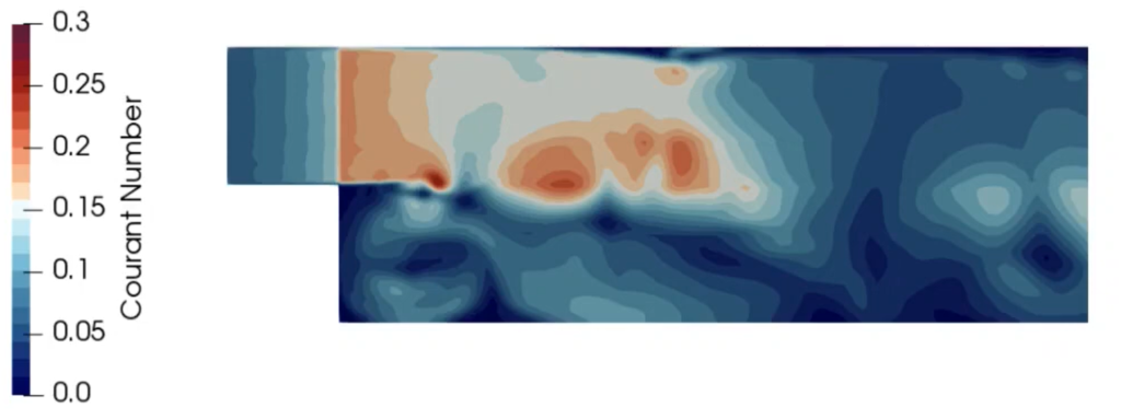
Figure 8- The Courant number field

How to calculate the Courant number in ANSYS Fluent?

To calculate the Courant number in ANSYS Fluent, you can visualize it as a contour plot. Follow these steps (Fig.9):

Go to the Contours panel (as shown in the picture).
In the “Contours of” dropdown menu, select Cell Convective Courant Number.
Set other options like “Filled” or “Node Values” as needed.
Click Compute to generate the plot.

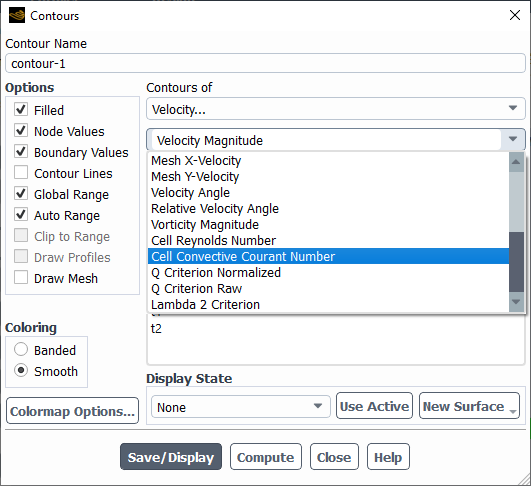
Figure 9- The schematic of Courant Number’s Contours setting in ANSYS Fluent

After setting the mentioned Cell Convective Courant Number in the Contours panel of ANSYS Fluent, you can visualize the Contours of Cell Convection Courant Number across the computational domain. This visualization helps identify areas where the Courant number may exceed stability limits, allowing you to refine the time step, mesh resolution, or solver settings to ensure numerical stability and accuracy in your simulation. (Fig.10).

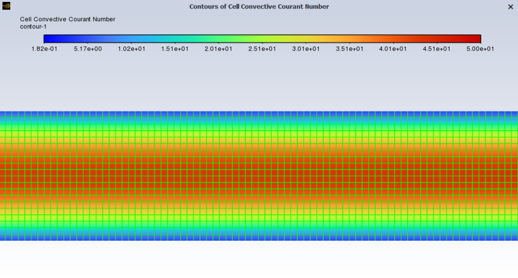
Figure 10- The schematic of Contours of Cell Convection Courant Number

Our ANSYS Fluent tutorial guides users through simulating heat-recirculating combustors with multiple injectors, focusing on thermal energy recovery to preheat incoming reactants (Fig.11). The tutorial employs a pseudo-transient method with careful Courant number management to ensure solution stability and accuracy.

Figure 11– Heat-recirculating Combustor with Multiple Injectors CFD Simulation – ANSYS Fluent Tutorial

Courant Number for Steady State and Transient Simulations

Courant Number for Steady-State Simulations

For steady-state simulations using the coupled solver, a high Courant number (default = 200)is typically used to accelerate convergence.
If the goal is accuracy, the Courant number should be less than 1.
If the goal is just to reach convergence quickly, a Courant number greater than 1can be used.

Courant Number for Transient Simulations

For transient simulations, the Courant number must typically be less than 1for numerical stability, with a recommended value of around 25 for accurate time-dependent simulations.
For specific cases, such as when no significant wave motion exists or the system is in a steady state, the Courant number can exceed 1. However, for most cases, keeping it below 10ensures better stability.
When using the VOF model, setting a global Courant number of 25ensures only 1 sub-time step is needed for VOF tracking, while a value of 1 will require 4 sub-time steps.

Understanding the Courant-Friedrichs-Lewy (CFL) number is essential in computational fluid dynamics (CFD) simulations. In transient simulations, such as the “Savonius Wind Turbine Using 6DOF Dynamic Mesh CFD Simulation” tutorial (Fig.12), managing the CFL number is crucial for numerical stability and accuracy. In contrast, steady-state simulations, like the “Gas-liquid Cylindrical Cyclone Separator CFD Simulation” tutorial (Fig.13), are less sensitive to the CFL number, but adjusting it can influence convergence rates. Our tutorials provide practical insights into handling the CFL number in both steady-state and transient CFD simulations.

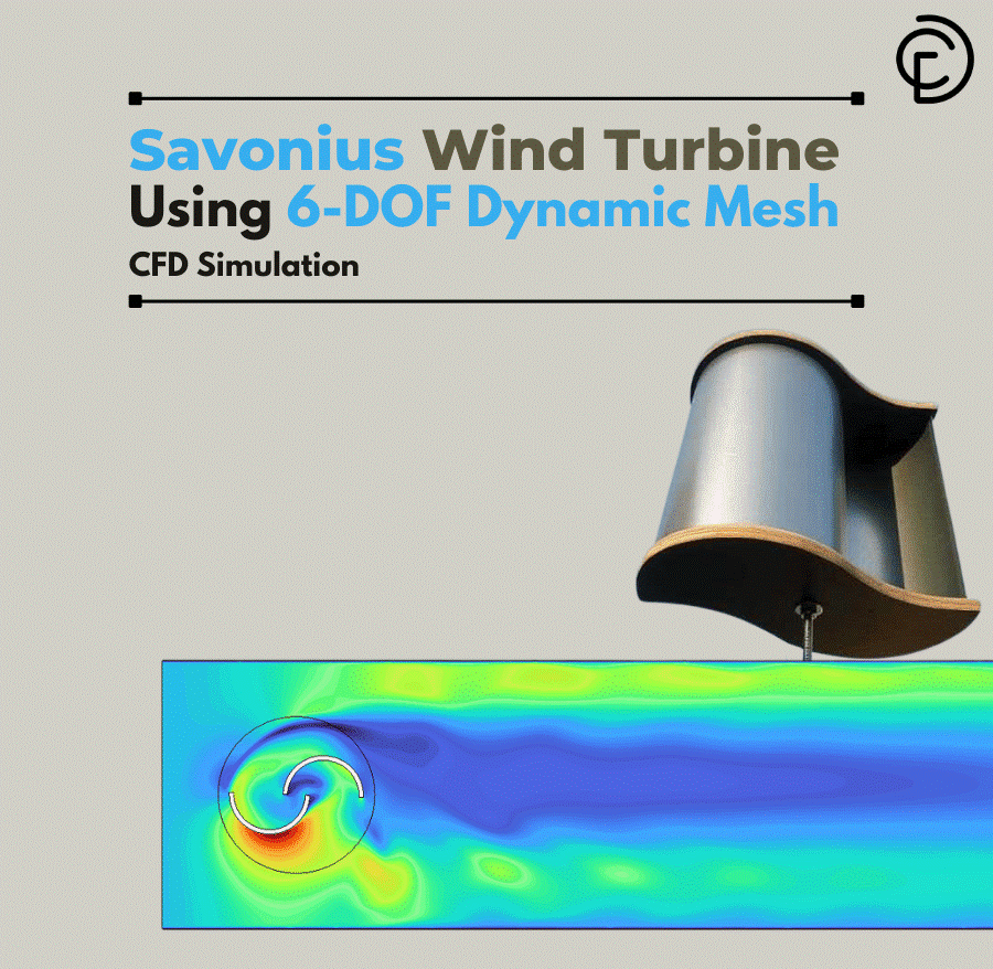
Figure 12– Savonius Wind Turbine Using 6DOF Dynamic Mesh CFD Simulation

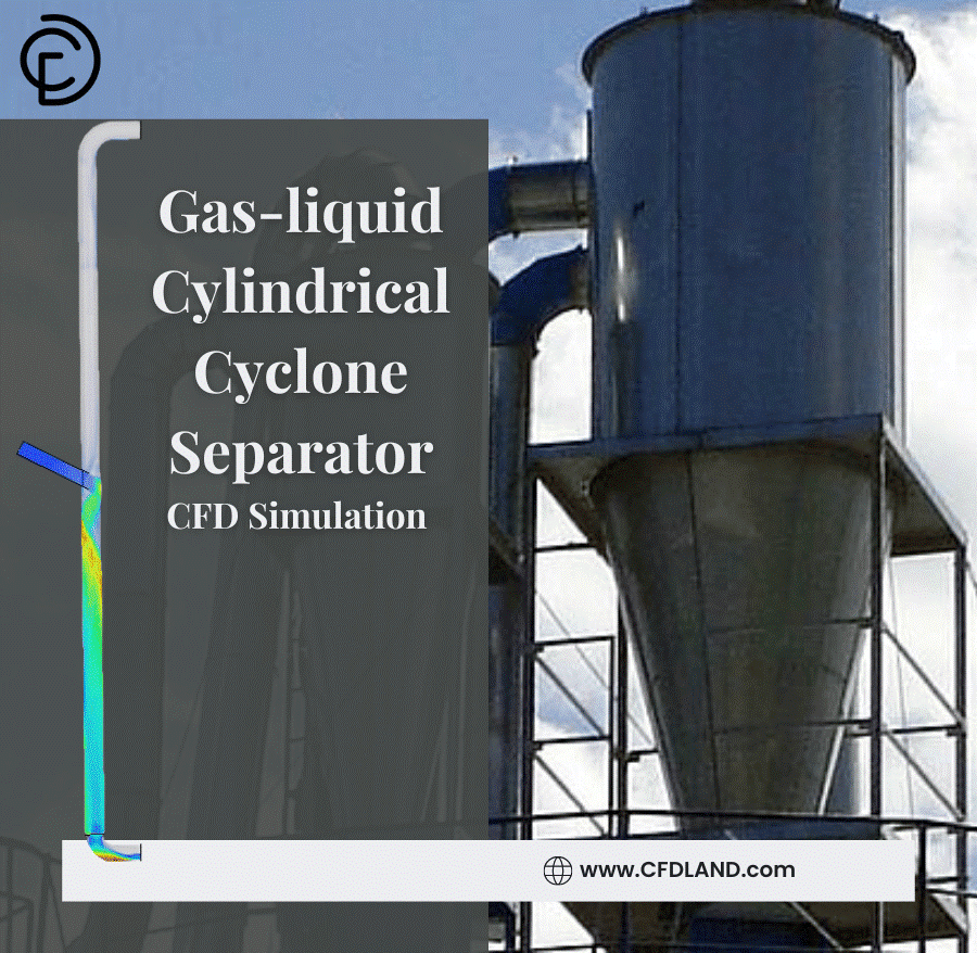
Figure 13– Gas-liquid Cylindrical Cyclone Separator CFD Simulation, ANSYS Fluent Training

Steps to Set the Courant Number in ANSYS Fluent

Step 1: Go to Solution Controls > Solution Methods panel > locate the Courant Number setting (Fig.14).

Step 2: Adjust the Courant number value based on the stability and accuracy requirements of your simulation.

For explicit solvers, keep it ≤ 1 for stability.
For implicit solvers, higher values (e.g., 5–50) may be used.

Step 3: Refine Time Step (if needed) – If the simulation is unstable, reduce the Courant number or adjust the time step size. The formula for adjustable time stepping is:

$\Delta t_{\text{new}} = \Delta t_{\text{old}} \cdot \frac{Co_{\text{max}}}{Co}$

Here, Co is the current Courant number, and Co,max is the maximum allowable Courant number.

Step 4: Run a Test Simulation – Monitor residuals and ensure numerical stability before proceeding with full-scale simulations (Fig.15).

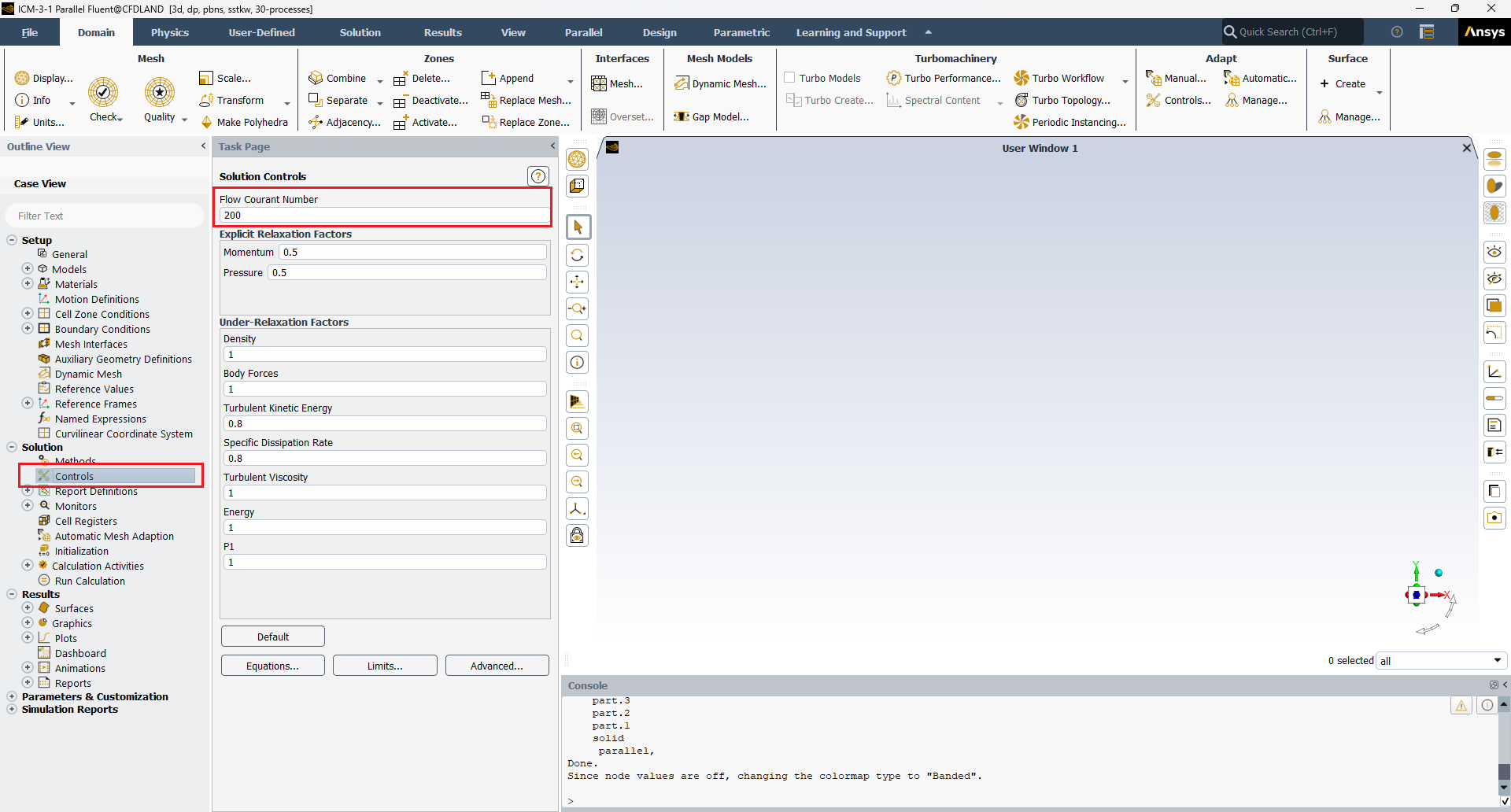
Figure 14- The Schematic of Solution Control in ANSYS Workbench

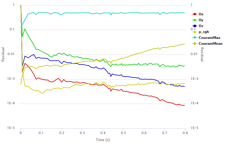
Figure 15- Convergence plot showing the selected Courant number is appropriate

Conclusion

The Courant number, also known as the CFL (Courant-Friedrichs-Lewy) number, is a key parameter in CFD that governs the stability and accuracy of numerical simulations. In explicit methods, the Courant number must typically remain ≤1 for stability, while implicit methods allow larger values, often exceeding 1. Applications of the Courant number extend to various CFD platforms such as OpenFOAM, HEC-RAS, and ANSYS, where it is calculated locally for each cell and visualized as a Courant number field. The CFL condition ensures that information does not travel more than one cell per time step, and violations can lead to instability or divergence. For example, in the VOF (Volume of Fluid) model, a global Courant number of 0.25 ensures stability with fewer sub-time steps. Overall, the Courant number calculation is essential in CFD for balancing simulation speed, accuracy, and stability across various solvers and scenarios.

FAQs

What is the Courant Number?

The Courant number (CFL number) is a dimensionless parameter in CFD that ensures numerical stability by determining how far information propagates in one time step relative to the grid size.

Is there a difference between Courant number and CFL number?

Courant Fredrich Lewy number (CFL) / Courant number, both are same. Just different packages use different ways of calling it.

How is the Courant number used in HEC-RAS?

In HEC-RAS, the Courant number is used to ensure stability in unsteady flow models. It must generally remain ≤ 1 for explicit solvers, but implicit solvers allow larger values.

What is the Courant number in OpenFOAM?

In OpenFOAM, the Courant number is calculated locally for each cell and visualized as a field. It dynamically adjusts the time step to maintain stability.

What is the Courant number for steady-state simulations?

For steady-state simulations, a high Courant number (e.g., 200) is used to accelerate convergence. For accuracy, the Courant number should be < 1.

What is the Courant number for transient simulations?

For transient simulations, the Courant number must typically be < 1 for stability, with 0.25 recommended for accurate time-dependent simulations.

Can you give a Courant number example?

Case 1:C=0.3: Stable, flow moves 30% of a cell in one time step.
Case 2:C=1.1: Unstable, flow moves more than a full cell, violating the CFL condition.