

Ansys fluent convergence is achieved when residuals fall below a set threshold and monitored physical quantities stop changing. Fluent’s default Ansys convergence criteria is 1e-3 for all equations and 1e-6 for energy; however, most engineering cases need 1e-4 to 1e-5 to ensure reliable results.
What Is Convergence?
If you are wondering what is convergence in CFD, it is the point where the iterative solution stops changing between computational cycles. Because CFD problems are non-linear, solving them requires an iterative process that gradually refines the solution. Successful convergence in CFD is reached when the numerical equations stabilize, and further iterations do not produce any meaningful change in the results.
To understand what is convergence in Ansys through a simple mathematical analogy, consider the limiting behavior of a sequence. A simple example is:
\frac{1}{2}, \frac{1}{4}, \frac{1}{8}, \frac{1}{16}, \frac{1}{32}, …
Each term in the sequence is half of the previous one. As you keep going, the terms get smaller and smaller, approaching zero. Even though no term in the sequence is exactly zero, the sequence converges to zero because, no matter how small an accuracy you choose, there will always be a point in the sequence where all following terms are within that accuracy from zero.
What Is the Difference Between Consistency, Stability, and Convergence?
These requirements, consistency, stability and convergence, define essential properties of numerical methods. They ensure accurate, reliable solutions by linking the numerical and analytical equations, preventing errors, and maintaining stability in simulations.
- Consistency: ensures the numerical method approximates the governing equations correctly, when time and space steps tend to zero. (Fig.1).
- Stability: ensures namely that all errors, such as round-off errors during computations do not grow uncontrollably (Fig.2), or remain bounded when the iteration process advances.
- Convergence: ensures the solution approaches the exact solution as the mesh and time step are refined or when time and space steps tend to zero. (Fig.3).
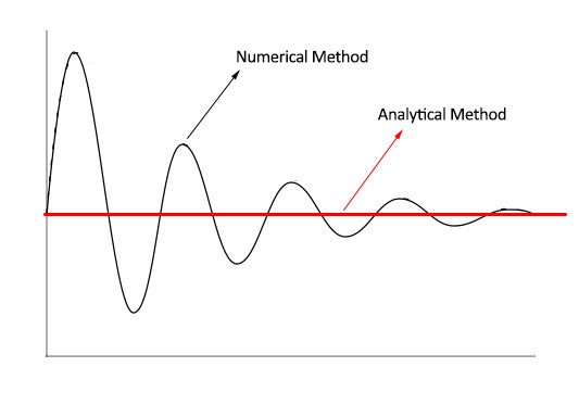
Figure 1- Consistency: The numerical method is limited to the governing equations during the marching of the solution.
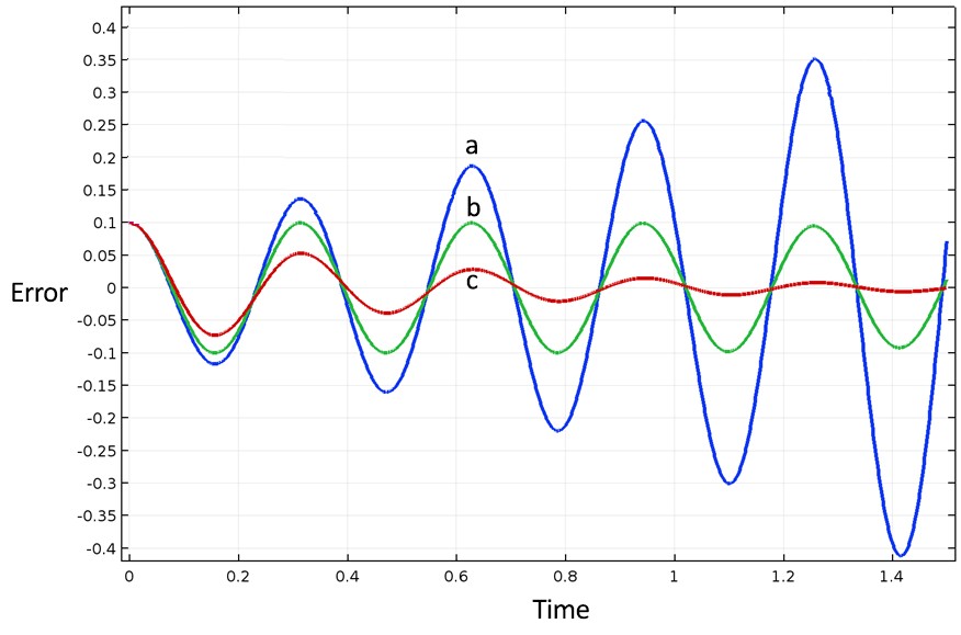
Figure 2- Stability: While (b) and (c) are reaching stability (b has bounded error), (a) is unstable.
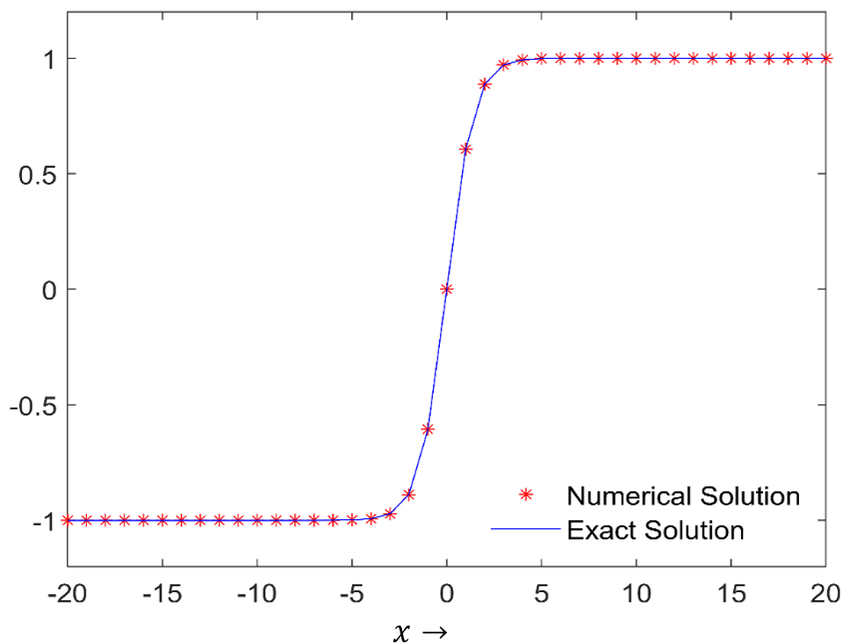
Figure 3- Convergence: the solution approaches the exact solution.
According to the Lax Equivalence Theorem:
“Consistency + Stability = Convergence”
Therefore, both consistency and stability are prerequisites for achieving convergence in numerical simulations. Fig.4 shows the ANSYS Fluent convergence conditions simply.
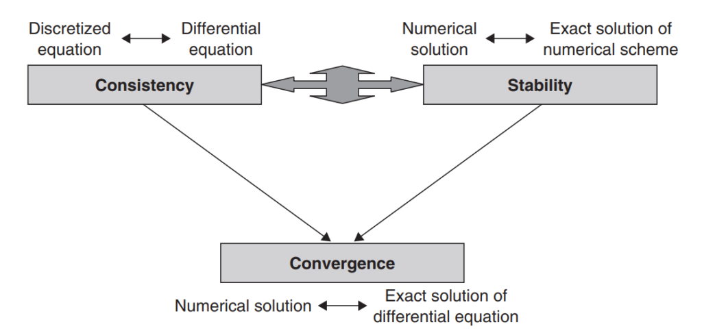
Figure 4- Relations between consistency, stability and convergence
How Residuals Indicate Convergence
Residuals in ANSYS Fluent measure how much the solution changes between iterations. Think of them as error indicators that tell you how far your current solution is from being fully solved (Fig.5). Although residuals are affected by numerical errors, low residuals do not always mean low numerical error; it’s important to check mesh quality and physical results to ensure an accurate solution. For a full breakdown of residual types, scaling, and monitoring, see our complete guide on residuals in ANSYS Fluent.
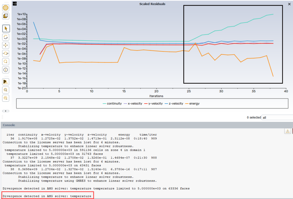
Figure 5- Residuals in ANSYS Fluent
What Convergence Criteria Value Should You Use?
Convergence criteria in ANSYS Fluent are essential to ensure that a CFD solution is stable and reliable. One of the primary indicators of Ansys fluent convergence criteria is the drop in residual values. But what exact value should you target?
| Case type | Recommended criterion | Notes |
|---|---|---|
| Fluent default | 1e-3 (energy 1e-6) | Too loose for most real cases |
| General steady flow | 1e-4 | Acceptable if monitors are flat |
| Heat transfer / species | 1e-5 – 1e-6 | Energy needs tighter criteria |
| Aerodynamics (Cd, Cl) | 1e-5 + force monitors | Residuals alone insufficient |
| Transient | Not residual-based | Use per-time-step convergence |
So, is an Ansys convergence criteria 1e-4 good enough? Yes, for most steady incompressible flows, provided your monitored quantities are flat and the mass balance closes.
As you can see in Fig.6, the left plot, labeled “Not Good Convergence,” shows residuals for Ux, Uy, Uz, k, and ϵ initially decreasing but stagnating or oscillating after around 300 iterations. More iterations are needed to reduce residuals further and achieve good convergence similar to the right plot, where residuals consistently drop below 1e-6.
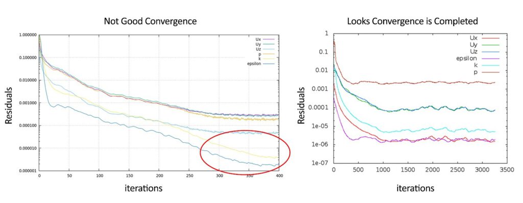
Figure 6- Comparison of residuals: incomplete vs. completed convergence
Stability of Key Monitored Variables
Apart from residuals, monitoring key physical parameters such as outlet velocity, pressure, mass flow rate, and temperature in a desired point, surface, etc. is essential (Fig.7). If these values fluctuate significantly, the solution is likely not yet converged.
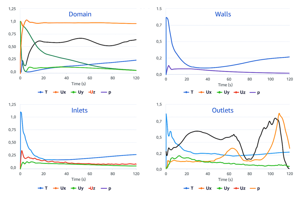
Figure 7- Stability of key monitored variables in a desired point and surface
Mass Balance
For many engineering problems, checking the balance of mass, momentum, and energy is a good convergence indicator. In a steady-state flow, the total mass flow rate at the inlet and outlet should be nearly equal (Fig.8). Energy balance also is maintained in heat transfer problems.
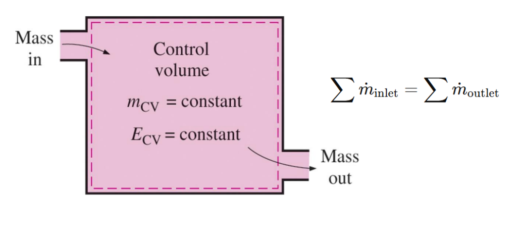
Figure 8- Mass balance in a steady flow control volume
Force Monitors (Drag and Lift Stability)
For aerodynamic simulations, monitoring drag and lift forces is a crucial part of CFD convergence criteria (Fig.9). If these values fluctuate excessively, additional iterations may be necessary.
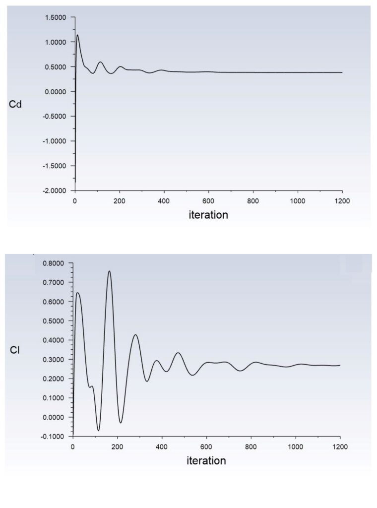
Figure 9- Drag (Cd) and Lift (Cl) coefficient stability after more than 1000 iteration
Lift-Drag Optimization on Airfoil using Mesh Morphing (Fig.10) is an ANSYS Fluent tutorial in which drag and lift stability play a crucial role. What we aim to do in this study over the base airfoil is to enhance the lift-to-drag ratio using the mesh morphing technique in ANSYS Fluent.

Figure 10- Lift-Drag Optimization On Airfoil Using Mesh Morphing (RBF)
How to Set Convergence Criteria in ANSYS Fluent
Setting appropriate convergence criteria ensures accurate and reliable results. Follow the below steps to set convergence criteria (Fig.11).
- Step 1: Access Residual Monitors. Navigate to Solution → Monitors → Residual → Edit.
- Step 2: Enable Convergence Monitoring. Check the boxes under the Monitor column and ensure Check Convergence is selected.
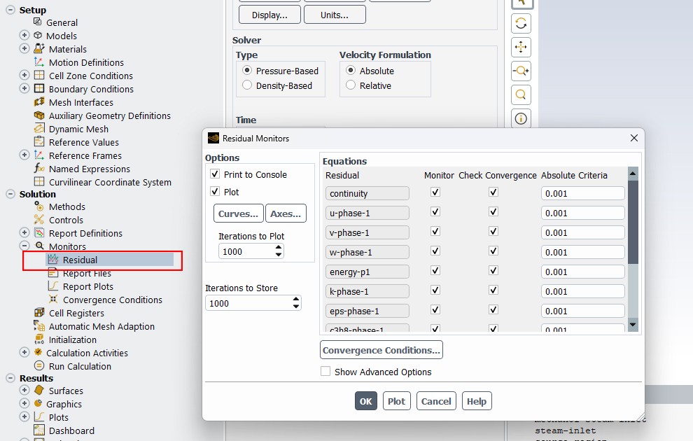
Figure 11- The schematic of residual monitor’s panel in ANSYS Fluent
- Step 3: Set Absolute Convergence Criteria. In the Absolute Criteria column, specify the threshold residual value for each equation (Fig.12). Lower values (e.g., 1e-6) indicate higher accuracy but may require more iterations.
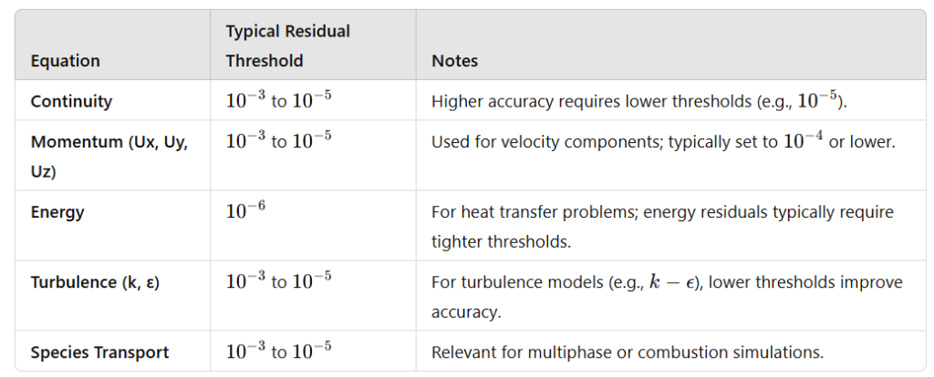
Figure 12- Common convergence criteria values in ANSYS Fluent
- Step 4: Plot Residuals.
- Step 5: Set Iterations to Plot and Store.
- Step 6: Convergence Conditions. Define additional criteria based on physical parameters.
- Step 7: Advanced Options. Enabling “Show Advanced Options” reveals settings like Normalize, Scale, Compute Local Scale, and Renormalize. Note: Scaled residuals are Fluent’s default and are what you generally compare against the 1e-3 threshold, whereas Normalize is useful if you need to compare residuals across different equations.
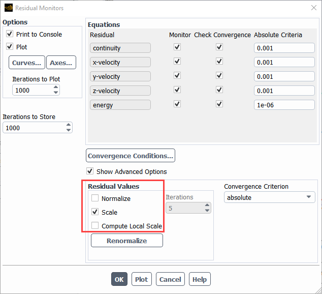
Figure 13- Enabling “show advanced options” in residual monitors’ panel
- Step 8: Apply and Start. Click OK to save the settings, and run the simulation.
Why Is ANSYS Fluent Not Converging? (7 Fixes)
If you are asking why is my simulation not converging, the issue usually lies in user setup errors rather than the solver itself. When you encounter the Ansys fluent not converging problem, check these seven critical areas:
- High Courant Number: In transient or density-based solvers, a time step that is too large causes instability. Reduce the time step.
- Poor Mesh Quality: High skewness or severe aspect ratios destroy stability. Ensure smooth cell transitions and review your grid in CFD Mesh Types before solving.
- Wrong Boundary Conditions: Using incompatible setups, such as placing a pressure outlet immediately next to an outflow, causes divergence. Read our guide on boundary conditions in ANSYS Fluent to ensure physical accuracy.
- Under-Relaxation Factors Too High: If variables update too aggressively, the solution will oscillate. Lower your URFs for pressure and momentum.
- Bad Initialization: A poor initial guess forces the solver to handle massive gradients in the first iteration. Use Hybrid Initialization instead of Standard.
- Inappropriate Pressure-Velocity Coupling: For highly swirling or complex flows, switch from the SIMPLE algorithm to the Coupled solver.
- Activating All Physics at Once: Do not turn on multiphase, heat transfer, and reactions simultaneously. Solve the cold flow first, then stage the remaining physics.
Convergence in Transient Simulations
Evaluating transient convergence Ansys fluent requires a fundamentally different approach than steady-state cases. In transient runs, convergence is evaluated per time step, not globally. When a new time step begins, residuals will spike upwards, and they must drop back down within that specific time step.
To successfully stabilize transient residuals CFD, you must set an appropriate number of iterations per time step—typically a maximum of 20 to 30. If the inner iterations fail to converge within that limit, you must reduce your overall time step size. Furthermore, do not rely on residuals alone. You must monitor a physical quantity (like average temperature or mass flow) over time to ensure the transient behavior is physically sound.
ANSYS Fluent Mesh Convergence
Mesh convergence in ANSYS Fluent refers to the process of ensuring that the numerical solution of a computational fluid dynamics (CFD) simulation is independent of the mesh size or grid resolution (Fig.14). In CFD, the physical domain is divided into smaller elements (mesh), and the accuracy of the solution can be significantly affected by how finely or coarsely this mesh is created.
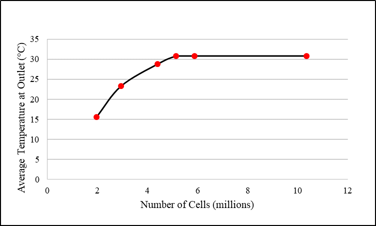
Figure 14- Grid independence test to ensure the mesh size
A practical example for understanding the better concept of grid independence test, is the CFDL tutorial: particle filtration DPM CFD simulation with Brownian force and UDF (Fig.15). This work examines the intricate dynamics of particle filtration via advanced CFD simulation utilizing ANSYS Fluent, specifically emphasizing the inclusion of Brownian force effects through User-Defined Functions (UDFs).
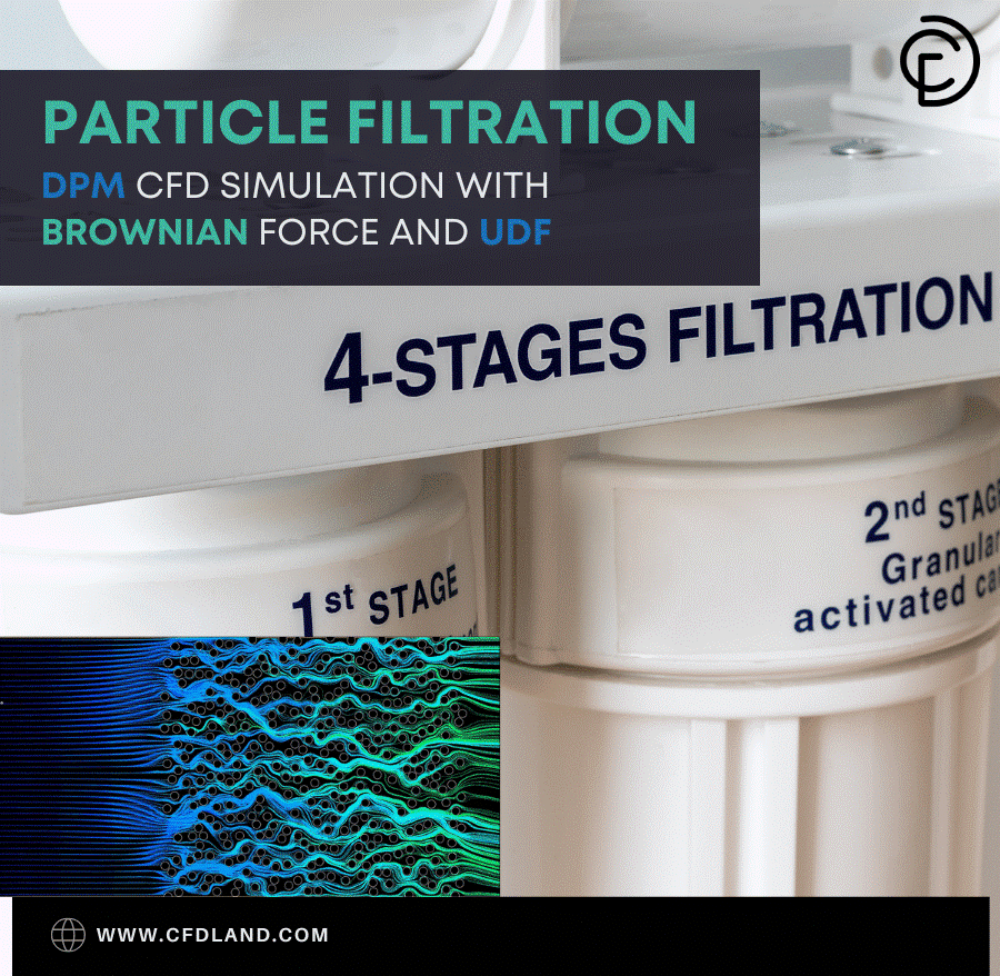
Figure 15- Particle Filtration DPM CFD Simulation with Brownian Force and UDF
Tips for Achieving Convergence in ANSYS Fluent
To improve convergence in ANSYS Fluent, consider the following tips:
- Domain Size: For external flows, set the outlet boundary 10× the characteristic length away (Fig.16).
- Solver & Material Properties: Use temperature-dependent density (Boussinesq) for natural convection to avoid divergence.
- Equation Discretization: For natural convection, use Body Force Weighted or PRESTO! for pressure instead of Standard.
- Step-by-Step Approach: In complex cases (e.g., boiling), first solve the flow field, then enable phase change without reinitialization.
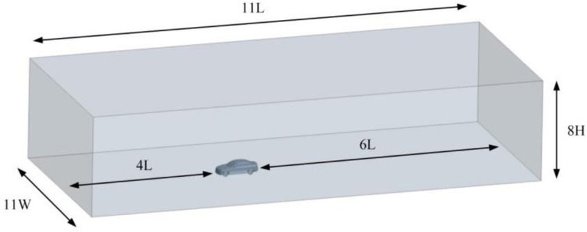
Figure 16- Recommended domain size for external flows
The aerodynamic analysis of Hatchback & Sedan cars CFD simulation is a free ANSYS Fluent training for better understanding of how to set appropriate domain size for external flows (Fig.17).

Figure 17- Aerodynamic analysis of Hatchback & Sedan Cars CFD simulation
Interpreting Convergence Messages in ANSYS Fluent
When running a simulation in ANSYS Fluent, users may encounter three key messages:
- Calculation is converged: This indicates that the simulation has successfully converged, meaning residuals have reached the user-defined threshold, and Fluent has stopped the solution.
- Calculation is completed: This message means the specified number of iterations has been reached, but it does not necessarily confirm convergence. The simulation may have stopped simply because the iteration limit was met.
- Calculation is diverged: This clearly indicates divergence. If this message appears, users should review boundary conditions, solver settings, mesh quality, and other aspects of the simulation to identify and fix the issue.
Sometimes, residual monitors may not reach our desirable values (e.g., stalling above 1e-3) and instead level off. However, if the simulation monitors appear flat, it does not necessarily indicate a lack of convergence. To ensure proper assessment, it is recommended to set up monitor points for parameters such as pressure and velocity at critical locations before starting the calculation. If these monitor points stabilize or exhibit a consistent oscillatory pattern over iterations, the simulation can be considered converged.
Conclusion
Convergence in ANSYS Fluent plays a pivotal role in ensuring the accuracy and stability of CFD simulations. By properly defining convergence criteria, refining meshes, and optimizing iteration strategies, users can enhance the reliability of their results. Addressing common challenges such as divergence and slow convergence requires a systematic approach, including monitoring residuals and adjusting solver settings. Mastering these techniques enables engineers to conduct more efficient simulations, leading to better-informed design decisions and improved computational performance. To see convergence handled correctly in complete, validated cases, browse our ANSYS Fluent tutorials.
FAQs
- What is convergence in ANSYS Fluent? Convergence in ANSYS Fluent occurs when numerical residuals stabilize below a specific threshold and key physical simulation parameters stop changing significantly.
- What is the default convergence criteria in ANSYS Fluent? The default convergence criteria ansys fluent applies is 1e-3 for continuity, momentum, and turbulence equations, and 1e-6 for the energy equation.
- Is 1e-4 a good convergence criterion in ANSYS Fluent? Yes, 1e-4 is an acceptable convergence criterion for most steady-state incompressible flows, provided your physical mass balance and surface monitors have also flattened out.
- How do I check if my simulation has converged? You can check if your simulation has converged by monitoring the steady drop in residuals, observing key physical flow parameters, and ensuring the mass, momentum, and energy balances are closed.
- Why is my simulation not converging? A simulation typically fails to converge due to poor mesh quality, incorrect boundary conditions, improper solver settings, or an excessive Courant number.
- What should I do if my residuals are oscillating? If your residuals are oscillating, you should refine the mesh, lower your under-relaxation factors, and double-check your boundary conditions for accuracy.
- How can I speed up convergence? You can speed up convergence by generating a high-quality orthogonal mesh, using Hybrid Initialization, and optimizing your solver settings such as switching to the Coupled solver.