
Imagine a large ocean wave hitting a ship’s hull, or water rapidly filling an empty tank. To study these physical events on a computer, you need a way to track the boundary between the water and the air. This is where the Volume of Fluid (VOF) model steps in. The volume of fluid method is a mathematical tool inside ANSYS Fluent designed specifically to simulate free surface flows. It calculates precisely where a liquid ends and a gas begins. Throughout this guide, you will learn how this approach works, when it makes sense to use it, and how to set up the mathematical schemes to get a sharp, accurate fluid boundary.
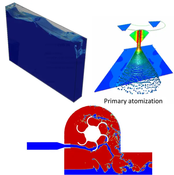
Figure 1: Common applications of the VOF model, showing clear boundaries between two fluids.
What is Multiphase Flow in CFD?
In fluid phase modeling, this condition happens when two or more distinct materials travel together through the same system. You might see gas and liquid acting together, like air bubbles in water. Sometimes it is two liquids, such as oil and water, or even solid particles moving inside a fluid. Because CFD software offers many ways to calculate these mixtures, picking the correct solver takes careful thought. If you want to know how to select the best mathematical approach for your project, read our complete guide on choosing a multiphase model.
Alternatively, if you want to understand the physical shapes these moving materials create such as bubble flow, slug flow, annular flow and more, you can see our guide on two-phase flow regimes. We`re not going to expand them here.
What is the VOF Model in CFD?
People often ask, what is VOF? In simple terms, VOF stands for Volume of Fluid. It is a specific mathematical technique used to track the boundary between two or more fluids that do not mix.
Originally introduced by Hirt and Nichols as a method for the dynamics of free boundaries, this approach operates on a fixed computational grid. When you set up a VOF simulation, the software looks specifically at the position of the interface dividing the materials.
The VOF method relies on four main characteristics:
- Shared Momentum: Instead of calculating separate movement rules for each material, the fluids share a single set of momentum equations.
- Volume Fraction Tracking: The solver checks every individual cell in the grid to calculate exactly how much of each phase sits inside it.
- Sharp Interface: The model draws a very thin, distinct boundary between the immiscible materials rather than blending them together.
- Mass Conservation: The equations ensure that no fluid volume disappears or is falsely created as the simulation runs forward in time.
When to Use VOF Model?
Knowing exactly when to apply this mathematical approach saves both time and computing power. The setup works perfectly for immiscible fluids, meaning liquids and gases that naturally refuse to mix. However, the software needs the right physical scale to calculate the boundary properly. You should base your decision on one simple rule: the interface length scale has to be larger than your computational grid. If your mesh cells are smaller than the fluid boundary you want to capture, the software will draw a sharp, accurate shape. For example, a large wave rolling over a ship spans thousands of cells, making it a perfect fit.
Conversely, the method breaks down if the fluid features become too small. If you try to simulate thousands of tiny, dispersed droplets that are smaller than your mesh cells, the solver cannot draw their borders. For those dense, small-scale conditions, you will need to switch to a different approach. You can read our complete guide on choosing the right multiphase model to see when Eulerian or Mixture setups work better. Finally, this setup cannot simulate two interacting gas phases. Gases mix at the molecular level, so they never form the physical wall required for this mathematical approach.
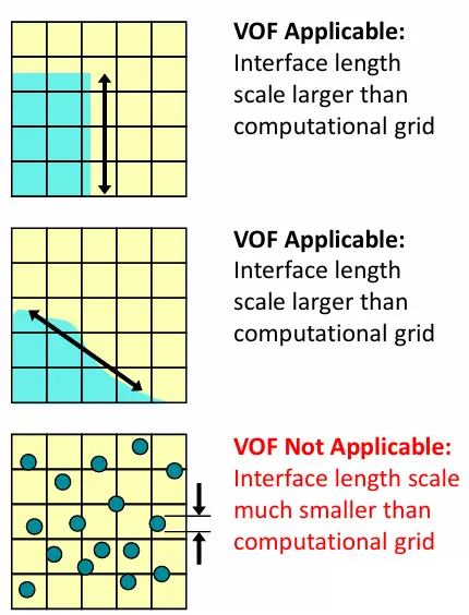
Figure 2: The physical applicability of the VOF multiphase model based on grid size.
Common Applications
Engineers rely on this method across many different industries. Because it excels at tracking physical boundaries, you will find it in almost any project involving a free surface. To make these examples easier to understand, we can group them into four main areas:
- Marine and Environmental: Designers use it to study wave-structure interactions, simulate open channels, and predict water movement.
- Tank Dynamics: It is the standard choice for calculating tank sloshing in moving vehicles or predicting liquid-liquid separation in oil refineries.
- Sprays and Injections: You can track jet breakup and initial atomization, where a solid stream of liquid shatters into smaller pieces.
- Industrial Components: It accurately captures the motion of large bubbles rising through columns. (Note: We will also explore cavitation here in our upcoming guide).
If you want to see how these projects look inside the software, you can explore our complete library of multiphase CFD simulation tutorials.
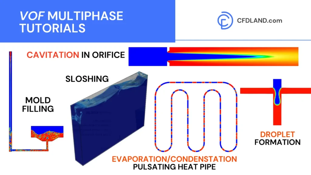
Figure 3: Practical examples of VOF multiphase CFD simulations from our shop library.
VOF Equations: The One-Fluid Approach
When running this solver, the software does not calculate separate movement rules for each material. Instead, it treats the mixture as a single effective fluid. This saves computing power, but it means both materials share the exact same velocity field. The governing equations are:
- Continuity equation for the mixture:
\frac{\partial \rho}{\partial t} + \nabla \cdot (\rho\mathbf{u}) = S_m
- Momentum equation for the mixture:
\frac{\partial (\rho\mathbf{u})}{\partial t} + \nabla \cdot (\rho\mathbf{u}\mathbf{u}) = -\nabla p + \nabla \cdot [\mu(\nabla\mathbf{u} + \nabla\mathbf{u}^T)] + \rho\mathbf{g} + \mathbf{F}_\sigma
- Volume fraction equation:
\frac{\partial \alpha_q}{\partial t} + \mathbf{u} \cdot \nabla \alpha_q = S_{\alpha q}
In these formulas, αq represents the volume fraction of a specific phase inside a cell. Its value always sits between 0 and 1. Furthermore, the sum of all fractions in a single cell always equals 1. Properties like density (ρ) and viscosity (μ) act as weighted averages based on how much of each material is present. By solving these equations step by step, the software tracks the overall volume of fluids moving through your domain.
In other words:
- αq represents the volume fraction of phase q
- 0 ≤ αq ≤ 1 with Σαq = 1
- Properties like density and viscosity are weighted averages based on volume fraction
Interface Tracking in VOF
The VOF method does not track the boundary as a physical mesh object. Instead, it relies on a volume-based system.
The solver looks at the liquid volume fraction (αl) inside every computational cell. If a cell has a value of 0, it contains only the secondary gas. If the value reads 1, it is completely filled with the primary liquid. The actual physical boundary exists only inside the cells that carry a value between 0 and 1.
To calculate this effectively, the interface tracking process follows three distinct steps:
- Representation: The solver records the fraction of liquid inside every cell.
- Interface Reconstruction: Using those fractions, the software calculates the slope and draws a flat line (or plane in 3D) inside each mixed cell to represent the boundary.
- Interface Movement: As time moves forward, the solver pushes these volume fractions into neighboring cells based on the local fluid velocity.
This step-by-step process allows liquids to naturally merge, deform, or break apart without needing special grid treatments.
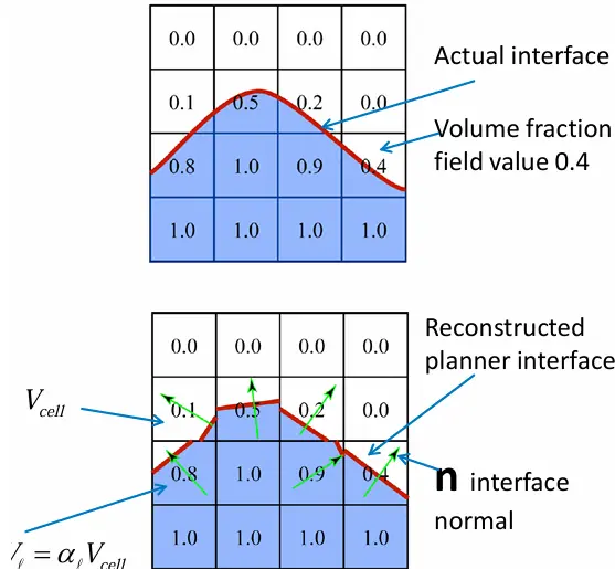
Figure 4: The three-step interface tracking process showing cell volume fractions and reconstruction.
Defining Phases in VOF Simulation – ANSYS Fluent
To set up a VOF model ANSYS Fluent simulation, you need to define three main parts. First, you assign the primary and secondary phases, which you can generally define in any order. Second, you input the material properties for each fluid. Third, you establish the initial conditions for the volume fractions inside your domain.
While the software gives you freedom in assigning these phases, a few tips help the solver run smoothly:
- It is safer to set your dispersed fluid, like isolated droplets or bubbles, as the secondary phase.
- If your setup includes a compressible ideal gas, you should set that gas as the primary phase. This choice provides better solution stability during the calculation.
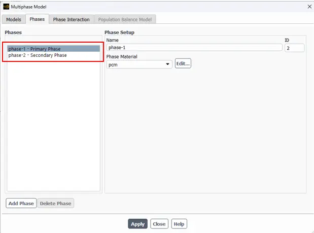
Figure 5: Setting up primary and secondary phases in the VOF Multiphase panel.
Explicit vs. Implicit Schemes for VOF
When adjusting your solver settings, one of the biggest choices is picking between the explicit vs implicit VOF formulations. The main difference lies in how the software calculates the volume fraction equation. If the solver uses values from the previous iteration, it runs the explicit method. If it uses values from the current iteration, it runs the implicit method. Each approach has specific benefits.
Explicit VOF Scheme: The explicit method reduces the computational cost per iteration, but it requires a much smaller time step. This scheme offers:
- Superior interface sharpness, especially when using the Geo-Reconstruct method.
- Better numerical accuracy overall compared to the implicit formulation.
- Excellent performance for surface tension-dominated flows.
- Availability only when the transient solver is turned on.
This method comes with strict time step limits based on the VOF Courant number. To maintain stability, ANSYS VOF automatically divides your physical time step into smaller pieces using this formula:
\Delta t_{Sub} = \text{Courant} \times \frac{\text{cell volume}}{\sum \text{outgoing fluxes}}
By keeping the Courant number below 1, you ensure the fluid boundary never crosses more than one cell per step, which protects the accuracy of your results.
Implicit VOF Scheme: The implicit formulation solves the phase continuity equation alongside momentum and pressure. This scheme provides:
- No Courant number limits, allowing you to use larger time steps.
- Full compatibility with both steady-state and transient calculations.
- Better computational efficiency for many industrial applications.
- Less accuracy in the interface representation because of numerical diffusion.
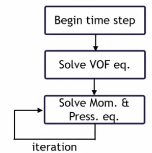
Figure 6: Explicit formulation in the VOF multiphase panel – ANSYS Fluent.
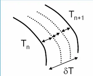
Figure 7: Interface location update during one time step – Explicit VOF formulation.
Interface Tracking Schemes and Accuracy
Interface Tracking Schemes and Accuracy
The physical accuracy of your fluid boundary relies directly on your chosen discretization method. The software provides different options depending on whether you use the explicit or implicit formulation.
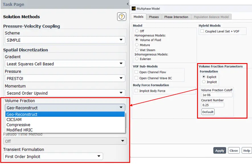
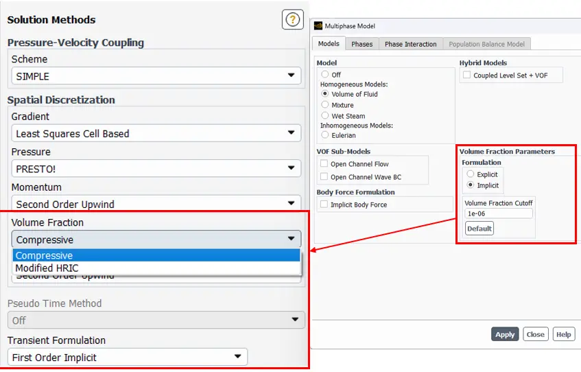
Figure 8: Available volume fraction discretization methods provided in ANSYS Fluent.
While the geo-reconstruct and compressive methods provide excellent accuracy, they do require more computing power than the simpler options. Knowing how these schemes compare helps you select the right tool for your specific multiphase problem:
- Geo-Reconstruct: This scheme delivers the sharpest interface representation across many different shapes, including circles and complex corners. It offers superior fidelity, but you can only use it with the explicit formulation.
- Compressive: The compressive scheme provides an excellent balance between accuracy and calculation speed. It works reliably in both explicit and implicit setups.
- CICSAM: The CICSAM scheme causes moderate interface smearing, but it handles complex geometric shapes quite well.
- HRIC: The HRIC scheme gives you much faster solution times, though it creates some extra numerical diffusion at the boundary.
Evaluating these trade-offs helps you capture the exact interface shape you need, whether you simulate simple bubbles or highly dynamic flows.
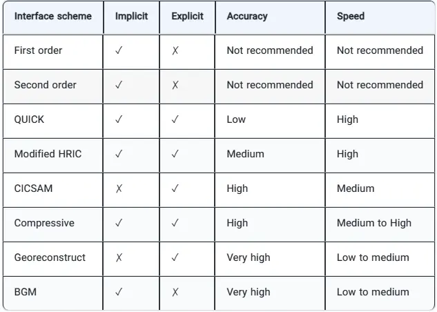
Figure 9: Interface tracking schemes provided in ANSYS Fluent – VOF multiphase modeling.
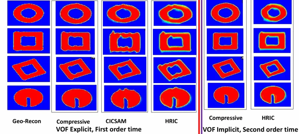
Figure 10: Visual comparison between volume fraction discretization schemes.
Steady-state VOF schemes
Running a calculation without tracking time saves massive amounts of computing effort. However, this steady-state VOF approach requires you to select a specific mathematical scheme to keep your fluid boundaries looking sharp instead of blurry.
Depending on your project goals, you can choose from three main options:
- Modified HRIC: This option delivers the fastest and most stable calculation. Engineers generally pick it for heavy industrial problems where overall speed matters more than perfect boundary thickness.
- Compressive Scheme: This acts as a reliable middle ground. It provides a highly practical balance of calculation speed, numerical stability, and boundary accuracy.
- BGM Scheme: The Bounded Gradient Maximization method represents the highest quality option for steady-state sharpness. It draws an extremely thin boundary, usually squeezing the transition into just a single mesh cell. While the BGM scheme takes longer to solve and requires careful setup to stay stable, it produces a crisp resolution that rivals transient calculations.
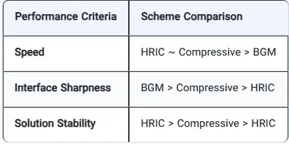
Figure 11: Comparison of discretization schemes for steady-state volume fraction modeling.
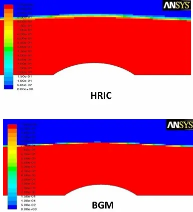
Figure 12: Visual comparison showing interface sharpness between the BGM and HRIC schemes.
Coupled Level Set VOF Method
Standard volume tracking perfectly conserves the physical mass of your fluids. However, it occasionally struggles to calculate the exact curvature of the fluid shape. On the other hand, the standard Level Set technique draws perfectly smooth curves but tends to lose fluid mass mathematically over time. To solve this, the solver offers the coupled level set VOF method. This hybrid tool blends both techniques together to eliminate their individual weaknesses.
The software uses the Level Set function to calculate the exact angle and curvature of the boundary line. At the exact same time, it uses the standard volume fractions to ensure no fluid mass disappears during the movement phase. This coupled approach requires more computing power, but it delivers incredible accuracy for small-scale physical problems. You will find it highly useful for simulating microfluidic devices, inkjet printer nozzles, or detailed bubble dynamics where the precise curvature of the droplet dictates the real-world physics.
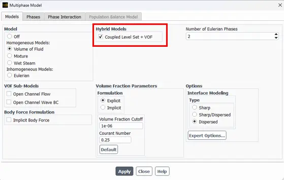
Figure 13: Activating the hybrid Coupled Level Set + VOF model in ANSYS Fluent.
Surface Tension and Wall Adhesion Modeling
When you model small bubbles, droplets, or microfluidics, physical boundary forces begin to control the flow. To capture these mechanics, you will choose the CSF or CSS model in the phase interaction panel.
Additionally, if your fluid touches a solid boundary, you need to activate wall adhesion to calculate how the liquid sticks to the surface. For a complete explanation of how to set up these specific forces, choose the right numerical model, and define your contact angles, read our complete guide on contact angle and surface tension.
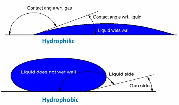
Figure 14: wall adhesion examples with hydrophobic and hydrophilic surfaces
Boundary Conditions For VOF Modeling
Defining physical behaviors at the edges of your computational domain dictates how your materials interact with the surroundings. When setting up VOF boundary conditions, you should ensure that only a single fluid phase enters or exits at any given inlet or outlet. To achieve this, set the volume fraction to 0 or 1 at these locations. For pressure inlets, patch the volume fraction to 1 in the cells sitting directly next to the boundary for the incoming phase. Furthermore, always set proper backflow values at your outlets. You should avoid using standard outflow boundaries altogether, as they frequently cause convergence problems in these setups.
Your starting state requires equal attention. You can generate clean initial conditions in three ways:
- Patching flow variables directly into specific fluid zones.
- Using volume registers generated through the Adapt tool.
- Selecting the patch reconstructed interface option to create a much sharper fluid boundary at the exact moment the simulation begins.
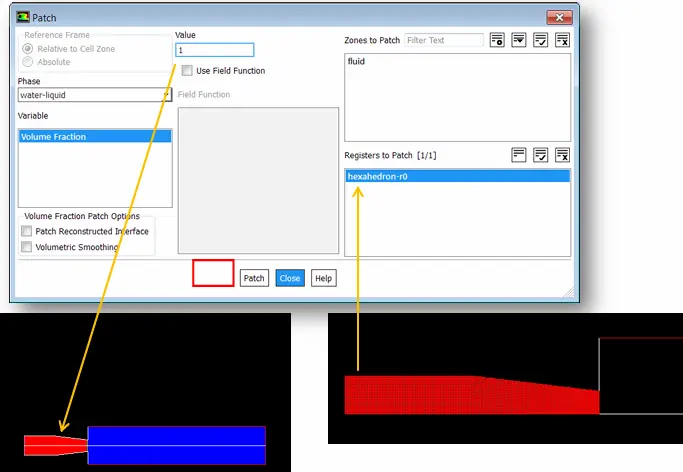
Figure 15: Patching the volume fraction during the initial setup.
Time Step Selection
The time step you choose directly influences the stability and physical accuracy of your numerical solution. A highly practical way to estimate a stable starting size relies on this formula:
\Delta t \approx \frac{1}{3} \times \frac{V_{cell,min}}{U}
In this equation, Vcell,min represents the smallest physical cell volume in your grid, which you can find in the Grid Check panel. The U variable represents the overall velocity scale of your problem, such as your main inlet speed.
As a general rule, you should start the run with a very small time step. After the solver completes a few initial calculations and the flow field stabilizes, you can safely increase the step size. If the calculation still fails or diverges, try opening the Solution Controls panel and turning off Skewness Neighbor Coupling.
Variable Time Stepping
To balance computational cost with precision, you can employ the variable time stepping technique. This tool allows the solver to automatically adjust the time step dynamically as the simulation moves forward. Instead of guessing a fixed value, the software monitors the global Courant number based on local flow conditions. If the flow accelerates rapidly, the solver reduces the time step. When the flow slows down, it increases the step size to speed up the overall calculation. You can set firm maximum and minimum limits for these adjustments, which optimizes your computational effort perfectly—especially when running explicit tracking schemes.
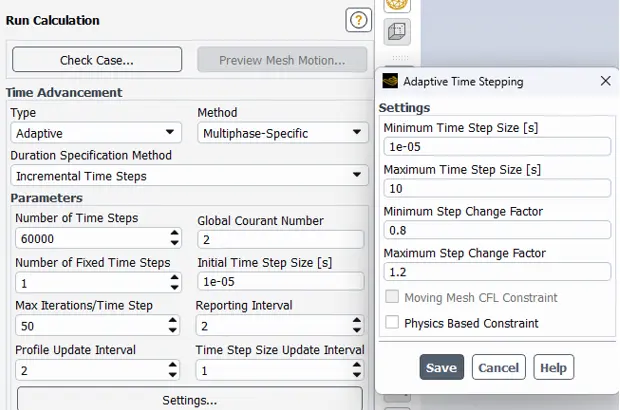
Figure 16: Activating the adaptive time stepping controls in ANSYS Fluent.
Multi-Fluid VOF Model
The multi-fluid VOF model operates as a hybrid between standard volume tracking and the Eulerian approach. You should use this option when your project requires separate velocity fields for every individual phase.
Instead of sharing one single momentum equation, the solver calculates completely separate velocity and temperature fields for each material. The software then models the physical interaction between these fluids using drag forces. Engineers find this specific setup highly useful for modeling industrial bubble columns that contain a large head space of gas at the top.
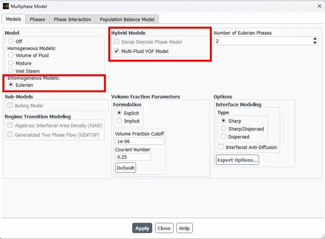
Figure 17: Activating the multi-fluid VOF model inside the ANSYS Fluent phase panel.
Open Channel Flow (VOF Sub-models)
When you simulate rivers, dam spillways, or irrigation channels, the standard solver needs extra boundary settings to capture the open air-water interface accurately. To solve this, the software offers a specialized open channel flow sub-model. This feature provides unique settings to handle wave propagation and define water heights at your inlets and outlets. However, setting up these specific hydraulic boundaries requires its own careful workflow. To learn how to define subcritical flows, establish wave boundaries, and use the 6DOF solver for floating structures, please read our dedicated guide on open channel flow simulation.
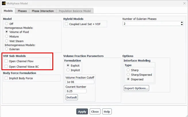
Figure 18: The open channel flow sub-model options in the VOF multiphase panel
VOF to DPM Model Transition
The VOF to DPM transition offers a hybrid approach for simulating liquid jet breakups. This method works in stages to handle spray physics efficiently without demanding an impossibly fine grid. First, the solver uses the standard volume tracking method to capture the flow near the nozzle and the initial droplet formation. As the simulation moves forward, the software automatically detects when droplets become too small for the mesh to resolve.
Instead of losing accuracy, the solver converts these tiny fluid pockets into Discrete Phase Model (DPM) particles. The software then continues tracking these newly formed droplets using Lagrangian particle equations. This transition saves massive amounts of computing power while maintaining physical accuracy. The hybrid setup also supports secondary breakup models and heat transfer effects, making it the best choice for fuel injection systems and industrial atomization processes. For instance, you can check two practical examples provided by CFDLAND team upon Jet in Crossflow for Aeronautical Applications and CFD Simulation of an Impinging Jet Spray which both benefit from VOF-to-DPM hybrid technique.

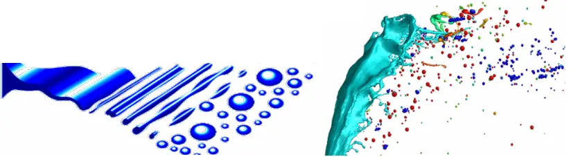

Figure 19: VOF to DPM transition occurring after the primary liquid injection.
Difference between VOF and Eulerian Models
You should use the Volume of Fluid method when your fluid interface is large enough for the mesh to resolve clearly. On the other hand, you should use the Eulerian model when your flow contains dispersed bubbles or droplets that are too small for your grid to capture. To learn exactly how to compare these setups and pick the right one for your project, please read our complete guide on choosing a multiphase model.
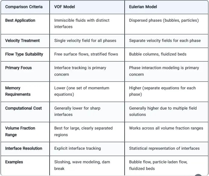
Figure 22: A summary comparison between models.
Conclusion
The Volume of Fluid technique gives engineers a highly reliable way to track sharp boundaries between different liquids and gases. Throughout this guide, we explored how to select the right volume fraction schemes, set up clean boundary conditions, and use hybrid tools like the VOF to DPM transition. By applying these specific tracking methods, you can simulate everything from small droplets to massive open channels with high physical accuracy. If you need expert help with your setup, you can easily order a CFD simulation project or book a CFD consultation with our engineering team today.
Frequently Asked Questions
- What is the Volume of Fluid (VOF) method?
The VOF method is a surface-tracking technique used in computational fluid dynamics. It calculates the exact shape and movement of a boundary between two or more fluids that do not mix, such as air and water.
- What is the VOF Courant number?
The Courant number is a stability limit used in explicit volume fraction calculations. It forces the solver to take smaller time steps so the fluid boundary never moves across more than one mesh cell during a single step, which protects the physical accuracy of the simulation.