
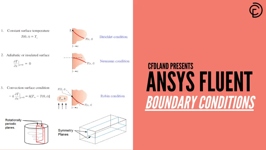
A boundary condition specifies the value or behavior of a flow variable at the edge of the computational domain. In fluid mechanics, boundary conditions in CFD constrain the discretized equations, ensuring the simulation accurately reflects real-world physics. Incorrect selection of these conditions will inevitably lead to physically impossible results, slow convergence or divergence.
Boundary Value Problem (BVP)
In mathematics and engineering physics, a Boundary Value Problem (BVP) refers to a differential equation (either ordinary or partial) that is solved along with specified boundary conditions at the domain boundaries (Fig.1). It should be noted that BVPs are different from Initial Value Problems (IVP), where the function’s value is given at an initial point rather than at the boundaries.
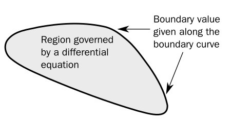
Figure 1- Boundary Value Problem Representation in a Computational Domain
Dirichlet, Neumann, and Robin Boundary Conditions
Understanding the fundamental types of boundary conditions is crucial for accurate simulation setup. In CFD, these are mathematically categorized into three primary types, alongside periodic conditions:
Dirichlet Boundary Condition
The dirichlet boundary condition specifies the value of the dependent variable at the boundary. In ANSYS Fluent, assigning a fixed velocity at an inlet or a constant temperature to a wall is a Dirichlet condition. These are also known as essential boundary conditions.
Neumann Boundary Condition
The neumann boundary condition specifies the derivative (gradient or flux) of the dependent variable at the boundary. Examples in Fluent include applying a specific wall heat flux, an adiabatic wall (zero heat flux), or an outflow/symmetry condition where gradients are zero. These are also known as natural boundary conditions.
Robin Boundary Condition
The robin boundary condition is a mathematical combination of Dirichlet and Neumann conditions. In Fluent, this is most commonly seen in thermal simulations where a convection wall is defined using both a heat transfer coefficient and a free-stream temperature.
| Type | Specifies | Mathematical form | Fluent equivalent |
|---|---|---|---|
| Dirichlet | Value of the variable | φ = φ₀ | Velocity inlet, fixed wall temperature |
| Neumann | Gradient / flux | ∂φ/∂n = q | Wall heat flux, adiabatic wall, symmetry |
| Robin | Combination | aφ + b ∂φ/∂n = c | Convection wall (h, T∞) |
| Periodic | Value repeats across boundaries | φ(x) = φ(x+L) | Translational / rotational periodic |
Fig.2 shows common types of boundary conditions in heat transfer. For example, setting an adiabatic boundary condition perfectly insulates a wall, meaning no thermal energy crosses the boundary (a zero-flux Neumann condition).
![Common Boundary Conditions in Heat Transfer[1]](https://cfdland.com/wp-content/uploads/2025/03/2-3.png "image of Boundary Conditions in CFD & ANSYS Fluent: All Types Explained")
Figure 2- Common Boundary Conditions in Heat Transfer [Fundamentals of Heat and Mass Transfer]
Boundary conditions physics define how a system interacts with its surroundings, and their mathematical classification—Dirichlet (fixed value), Neumann (fixed flux), and Robin (mixed condition)—directly corresponds to boundary types in ANSYS Fluent. For example, wall boundaries in Fluent can impose fixed temperature (Dirichlet), heat flux (Neumann), or convection (Robin). Similarly, velocity inlets and pressure inlets/outlets represent Dirichlet and mixed conditions, respectively. Fluent also includes symmetry and periodic boundaries, which align with Neumann-type constraints. Understanding these relationships ensures accurate boundary condition selection in CFD simulations, leading to more reliable results.
How to Set Boundary Conditions in ANSYS Fluent
Once you have your geometry and mesh prepared in ANSYS Meshing, follow these steps to learn how to give boundary conditions in ANSYS Fluent.
Step 1: Launch ANSYS Fluent
- Open ANSYS Fluent after meshing is complete.
- Set the solver type (pressure-based or density-based).
- Choose whether the simulation is steady or transient.
Step 2: Access the Boundary Conditions Panel (Fig.3)
- In ANSYS Fluent, go to “Setup” > “Boundary Conditions”.
- A list of boundary zones (inlet, outlet, walls, symmetry, etc.) will be displayed.
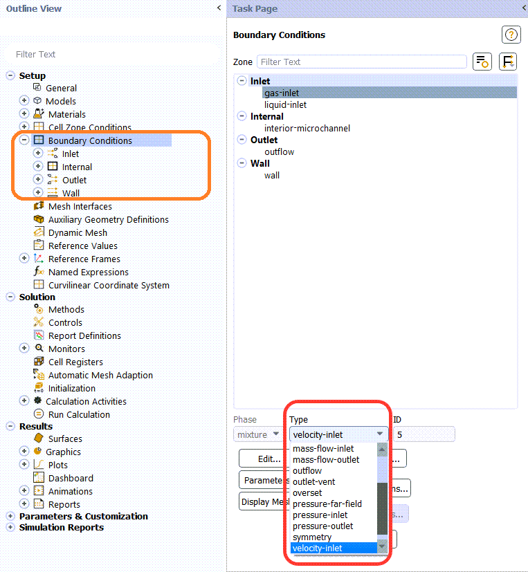
Figure 3- The Schematic of Boundary Conditions Panel in ANSYS Fluent
Step 3: Assign Boundary Types and Parameters (Fig.4)
- Click on a boundary zone (e.g., “inlet”).
- Select the appropriate boundary condition type (velocity, pressure, wall, etc.).
- Input relevant parameters such as:
- Velocity/Mass Flow Rate (for inlets)
- Pressure values (for pressure inlet/outlet)
- Wall temperature or heat flux (for heat transfer simulations)
- Turbulence parameters (if applicable, e.g., turbulence intensity, length scale)
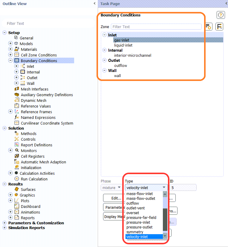
Figure 4- Boundary Conditions Example in ANSYS Fluent
Step 4: Set Additional Properties (if applicable)
If solving for heat transfer, you must define the ANSYS Fluent thermal boundary conditions. Based on the theory above, you can apply:
- Fixed Temperature: Defines a constant surface temperature (Dirichlet).
- Heat Flux: Defines a specific heat input or an adiabatic (zero-flux) boundary (Neumann).
- Convection / Mixed: Defines heat transfer via a free-stream fluid (Robin).
Step 5: Verify and Apply
- Ensure all boundary conditions are correctly defined. Click OK or Apply to save settings.
Types of Boundary Conditions in ANSYS Fluent
Overall, the boundary conditions in ANSYS Fluent can be categorized into External Boundaries and Internal Boundaries (Fig.5).
To quickly reference the appropriate boundary type for your simulation, use the classification table below:
| Category | Boundary condition | Use when |
|---|---|---|
| External – any flow | Pressure inlet / Pressure outlet | Pressure known, flow rate unknown |
| External – incompressible | Velocity inlet, Outflow | Velocity known |
| External – compressible | Mass flow inlet, Pressure far field | Compressible / external aero |
| External – other | Wall, Symmetry, Axis, Periodic | Geometry-driven |
| Special | Inlet/outlet vent, Intake/exhaust fan | Vent & fan systems |
| Internal | Interface, Fan, Interior, Porous jump, Radiator, Internal wall | Zero-thickness internal features |
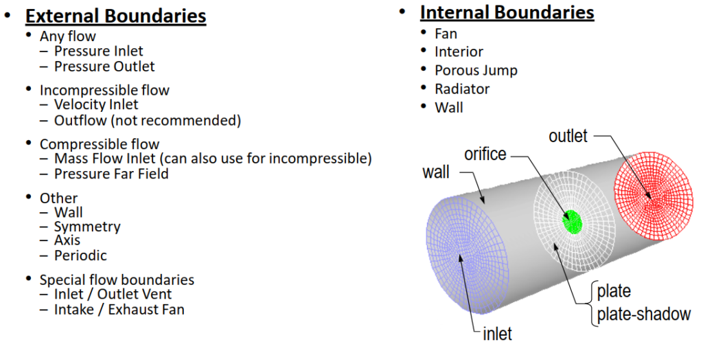
Figure 5- Types of Boundary Conditions in ANSYS Fluent
In the remainder of this blog, we examine these specific Ansys fluent boundary conditions in detail.
External Boundary Conditions
These boundary conditions define the interaction between the computational domain and its surroundings. External boundary conditions can be classified into:
Any Flow:
- Pressure Inlet: Specifies the pressure at the inlet boundary, commonly used in incompressible and compressible flows. Pressure inlet boundary conditions can be used when the inlet pressure is known but the flow rate and/or velocity is not known. This situation may arise in many practical situations, including buoyancy-driven flows. When setting this condition, you must also define the backflow volume fraction and turbulence parameters to prevent divergence if reversed flow occurs.
- Pressure Outlet: Defines the pressure at the outlet boundary, ensuring proper flow exit conditions (Fig.6). Non-reflecting outlet boundary conditions (NRBC) are available for ideal gas flow. It should be noted that Hydraulic Diameter in ANSYS Fluent is a key parameter used for flow analysis in non-circular ducts and complex geometries. To calculate it, you can easily use our Hydraulic diameter calculator FREE tool.
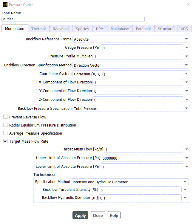
Figure 6- The Schematic of Pressure Outlet Boundary Condition in ANSYS Fluent
Incompressible Flow:
- Velocity Inlet: Specifies velocity and direction at the inlet boundary for incompressible flow scenarios (Fig.7). Velocity inlets apply a uniform velocity profile at the boundary unless a UDF is used. They are not recommended for compressible flows.
- Outflow: Allows flow to exit the domain without specifying values. This is less robust and typically avoided.
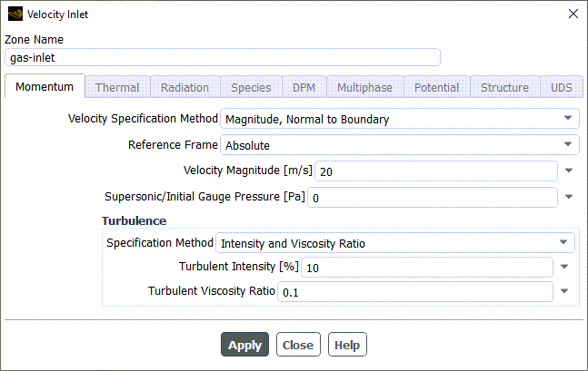
Figure 7- The Schematic of Velocity Inlet Boundary Condition in ANSYS Fluent
Compressible Flow:
- Mass Flow Inlet: Specifies the mass flow rate at the inlet boundary, suitable for compressible flows (can also be used for incompressible flows).
- Pressure Far Field: Used for external aerodynamic simulations, where the boundary is far from the object.
Wall Boundary Condition
The wall boundary defines a solid, stationary, or moving boundary within the domain (Fig.8). Thermally, an adiabatic wall can be applied here by setting a zero heat flux (Neumann condition).
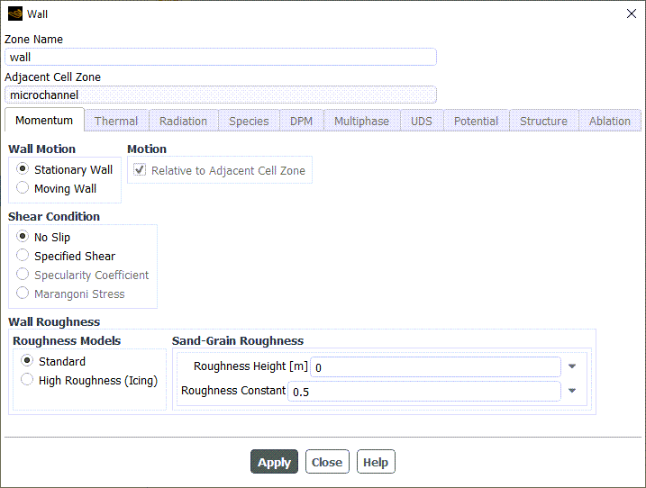
Figure 8- The schematic of Wall Boundary Condition in ANSYS Fluent
The wall settings allow users to define critical parameters for simulating fluid behavior near surfaces, including shear conditions, motion, and roughness (such as icing) for turbulent flows.
No-Slip and Slip Wall Boundary Conditions
In standard viscous flows, the no slip boundary condition is applied as the default state. This means that friction dictates the fluid velocity at the wall is exactly zero, ensuring an accurate representation of shear stress interactions. However, in highly rarefied gases or microfluidics where the Knudsen number is large, a slip boundary condition is required, allowing the fluid to slide along the solid surface with a non-zero velocity. For a practical demonstration, see our tutorial on Slip and Non-slip Flow inside a 2D Microchannel CFD Simulation.

Symmetry Boundary Condition
Used for domains with symmetric flow patterns, reducing computational requirements (Fig.9). The Fig.10 displays a dialog box for defining a Symmetry Boundary Condition in ANSYS Fluent. The Symmetry Boundary Condition is applied to ensure that the flow field and geometry remain symmetric, meaning no inputs are required. At the symmetry plane, the normal velocity must be zero, and all variables must have zero normal gradients. Proper definition of symmetry boundary locations is essential to maintain accurate and physically consistent simulation results.
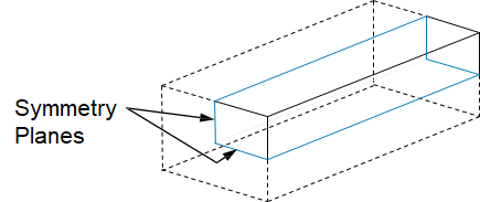
Figure 9- The Concept of Symmetry Boundary Condition
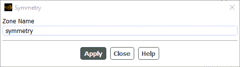
Figure 10- The Schematic of Symmetry Boundary Condition in ANSYS Fluent
Axis Boundary Condition
In ANSYS Fluent, the Axis Boundary Condition is used for 2D axisymmetric problems, where the centerline of the axisymmetric geometry is defined (Fig.11). No user inputs are required, but it is crucial that the axis boundary coincides with the x-axis to ensure accurate simulation results.
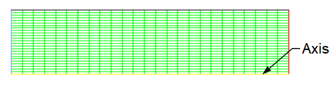
Figure 11- The Concept of Axis Boundary Condition
Compressible Flow In Nozzle CFD Simulation (Fig.12) is a CFD LAND product which enables you to understand the better conception of symmetry boundary conditions. Having split from the midplane, the Axisymmetric approach is applied to solve flow equations in a cylindrical framework.
Figure 12- Compressible Flow In Nozzle CFD Simulation, ANSYS Fluent Training
Periodic Boundary Conditions
A periodic boundary CFD setup is utilized when physical geometry and flow patterns repeat themselves in a cyclic manner, allowing engineers to simulate only a single repeating fraction of the domain to drastically reduce mesh size and solve time (Fig.13).

Figure 13- The Schematic of Periodic Boundary Condition in ANSYS Fluent
To set periodic boundary conditions in ANSYS Fluent, the flow field and geometry must exhibit either rotational or translational periodicity:
| Periodic Type | Pressure Requirement | Typical Use Case |
|---|---|---|
| Rotational | Pressure difference (ΔP) across planes is zero | Turbomachinery CFD Simulations, swirling flow in cylinders |
| Translational | Finite pressure difference allowed across planes | Fully developed pipe flows, heat exchangers |
When using translational periodicity, users must specify either the mean pressure difference per period or the net mass flow rate. The Fig.14 illustrates two types of periodic boundaries in fluid simulations. Part (a) shows a 2D tube heat exchanger with translationally periodic planes. Part (b) depicts a cylindrical configuration with rotationally periodic planes.
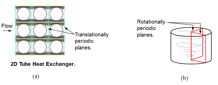
Figure 14- Periodic Boundary Conditions in Fluid Dynamics Simulations (a) 2D Tube Heat Exchanger with Translationally Periodic Planes (b) Cylindrical Geometry with Rotationally Periodic Planes
Erosion in Air-cooled Condenser (ACC) CFD Simulation (Fig.15), is a process that happens when water droplets or steam traveling at high speed strike the inside surfaces of condenser tubes, gradually releasing material. Utilization of periodic boundaries results in a thorough, computationally efficient analysis of the whole system.
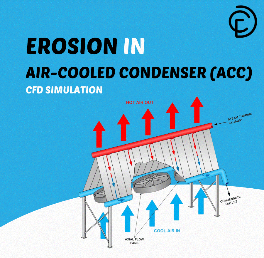
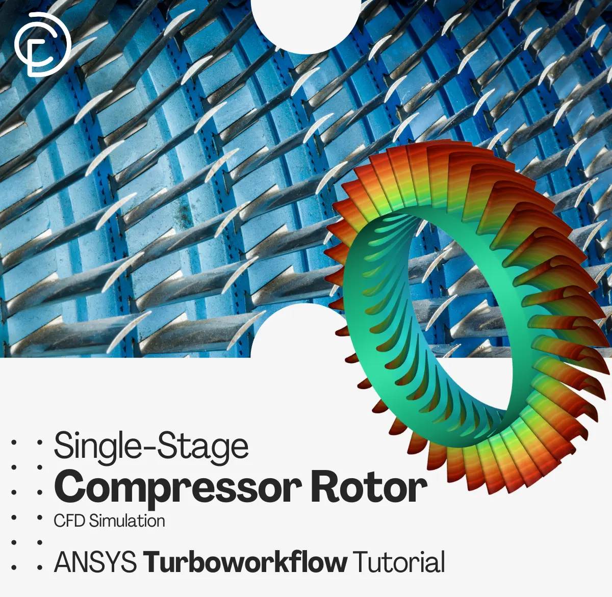
Figure 15- two great examples where periodic boundary condition saves time and cost
Another case in a point is Single-Stage Compressor Rotor CFD Simulation in which one blade inserted and multiplied in row with periodic condition.
Special Flow Boundaries
- Inlet/Outlet Vent: Simulates vent boundaries for intake or exhaust systems.
- Intake/Exhaust Fan: Models fan boundaries for flow intake or exhaust.
Internal Boundaries
Internal boundaries are used directly within the computational domain to model specific internal flow phenomena, abrupt condition changes, or physical features without requiring external inlets or outlets. Internal boundaries can be categorized into:
- Interface: Mesh interfaces are defined only on cell faces and have zero thickness, allowing for sudden changes in flow properties between adjacent zones (Fig.16). For mesh interface setup, non-conformal meshes, and sliding-mesh cases, see our complete guide on the interface boundary condition in ANSYS Fluent.
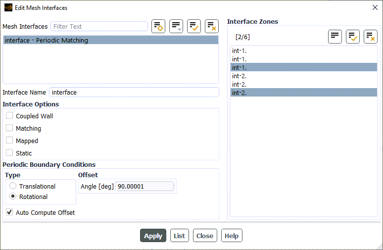
Figure 16- Edit Mesh Interfaces Tab in ANSYS Fluent
- Fan: Models fluid acceleration by assigning a specific pressure jump across a zero-thickness plane. Read our dedicated guide on the fan boundary condition.
- Interior: Represents internal regions of the mesh where fluid cells transition seamlessly without any barrier.
- Porous Jump: Simulates a thin membrane or screen where there is a pressure drop and velocity change across the boundary.
- Radiator: Models heat exchange or flow resistance in radiator-like geometries.
- Internal Wall: Internal walls can be defined for specific interactions within the domain, such as internal heat transfer or flow separation barriers.
Boundary conditions programming in ANSYS Fluent
When default settings are insufficient, you can program dynamic or highly complex constraints—such as a parabolic velocity profile or a time-varying temperature distribution—using a User Defined Function (UDF). By using the specific DEFINE_PROFILE macro, custom C-code can be compiled and hooked directly into the boundary condition panel to override standard solver behaviors.
For instance, Flow Inside a 2D Microchannel CFD Simulation mentioned above (Fig.17), is a CFDLAND project which study the difference the Slip or non-slip flow regime causes inside a microchannel. More importantly, a user-defined function (UDF) must be written to apply slip flow regime conditions to the microchannel walls because the ANSYS Fluent itself doesn`t have predefined governing equations.
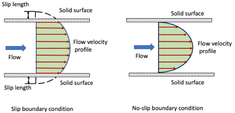
Figure 17- The changes in velocity profile on a slip wall must be modeled with a programmed boundary condition
Guidelines for Boundary Conditions and Grid Setup in Fluid Simulations
- Boundary Location and Shape: Select inflow and outflow boundary locations and shapes to ensure flow enters or exits normal to the boundaries for better convergence.
- Gradient Observation: Avoid large gradients in the direction normal to the boundary, as this indicates an incorrect setup. Adjust the boundary position further upstream or downstream to move away from gradients.
- Grid Skewness: Minimize grid skewness near the boundary to reduce numerical diffusion and prevent errors in simulation accuracy.
Conclusion
In conclusion, the proper selection and implementation of boundary conditions are fundamental for accurate and reliable CFD simulations in ANSYS Fluent. These conditions, which define how the computational domain interacts with its surroundings, directly affect the flow characteristics, convergence, and overall performance of the simulation. By understanding the various boundary condition types—including Dirichlet, Neumann, Robin, and periodic conditions—users can ensure that the flow physics are accurately represented. Furthermore, the use of UDFs enhances flexibility, allowing for highly customized parameters to be applied. To see these boundary conditions applied in complete, validated cases, browse our ANSYS Fluent tutorials.
FAQs
- What are boundary conditions in CFD? They define how fluids interact with the boundaries of the computational domain, ensuring accurate solutions.
- Why is it important to choose the right boundary condition? They are crucial for achieving accurate, stable, and converging simulation results.
- What is the difference between external and internal boundary conditions? External affects domain boundaries; internal applies to specific domain areas (e.g., porous media).
- How do I set boundary conditions in ANSYS Fluent? Select boundary zones, define type (e.g., inlet, outlet), and apply the parameters.
- Can I define custom boundary conditions? User Defined Functions (UDFs) allow custom boundary conditions via programming.
- What is the significance of symmetry boundary conditions? Used for symmetric flows to reduce computational effort.