Acoustics

What Exactly Are Acoustics and Aeroacoustics?

When we hear the word “sound,” we often think about music, voices, or even noises around us. But for engineers, sound is much more than that. It is a science that helps us understand how sound is created, how it travels, and how it is heard. This science is called acoustics, and it plays a very important role in designing quieter machines, safer workplaces, and more comfortable spaces.

Acoustics is the study of sound waves. A sound wave is created when an object vibrates, like the strings of a guitar or the engine of a car. These vibrations cause changes in air pressure, which we hear as sound. Acoustics focuses on how these sound waves move through different mediums, such as air, water, or solid materials. It also looks at how sound waves behave—how they reflect, absorb, or travel to reach our ears. In engineering, acoustics helps us solve problems like reducing noise in factories, improving music quality in concert halls, and controlling sound in offices or homes.

Figure 1: Visualizing the sources of sound in engineering acoustics. The field of Acoustics (left) often studies sound originating from structural vibration. In contrast, Aeroacoustics (right) focuses on sound generated directly by turbulent fluid flow.

On the other hand, aeroacoustics is a special branch of acoustics. It focuses on sound that is created by moving fluids like air or water. For example, the noise made by an airplane flying through the sky, the hum of a fan, or the sound of air rushing through a ventilation system are all examples of aeroacoustics. In these cases, the sound does not come from vibrations of solid objects. Instead, it comes from the movement of fluids and the turbulence they create. Engineers use aeroacoustics to study how air or water flows and how this movement creates sound. This helps them design quieter airplanes, better wind turbines, and more efficient ventilation systems. Both acoustics and aeroacoustics are important sciences that help engineers predict and control sound. Whether it is reducing noise pollution in cities or designing quieter machines, these fields are key to improving the way we live and work.

Core Concepts in Acoustics and Aeroacoustics

Acoustics is all about understanding how sound behaves. One of the most important concepts in acoustics is pressure fluctuation. Sound waves are actually changes in pressure that travel through air, water, or solid objects. Imagine dropping a pebble into water. The ripples spreading out are like the sound waves created by pressure changes. These waves have areas of high pressure (compression) and low pressure (rarefaction). This movement of pressure is what allows sound to travel from its source to the listener.

In engineering, pressure fluctuations are key to understanding how sound propagates, or moves, from one place to another. For example, in a factory filled with noisy machines, the sound travels through the air as pressure waves. Engineers study these waves to find ways to reduce noise levels. They may use materials that absorb sound or design machines that vibrate less. This is called industrial noise control, and it’s important for keeping workers safe and productive.

Figure 2: A visual bridge between aeroacoustics and musical acoustics, illustrating how the same physical principles of air movement and pressure waves govern both the roar of aircraft and the resonance of a guitar.

Aeroacoustics is the study of how sound is created by moving fluids, such as air or water. It links fluid dynamics—the study of how fluids move—with sound generation. This field helps engineers understand why noise is produced and how it can be controlled. For example, when air flows quickly over the wings of an airplane or through a ventilation duct, it creates turbulence. This turbulence leads to changes in pressure, which generate sound. The sound caused by moving fluids is called aeroacoustics noise.

One key part of aeroacoustics is fluid flow acoustics. This focuses on how the movement of air or water produces sound. For example:

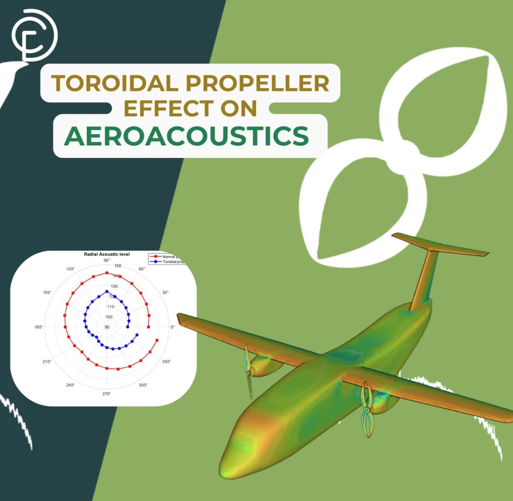
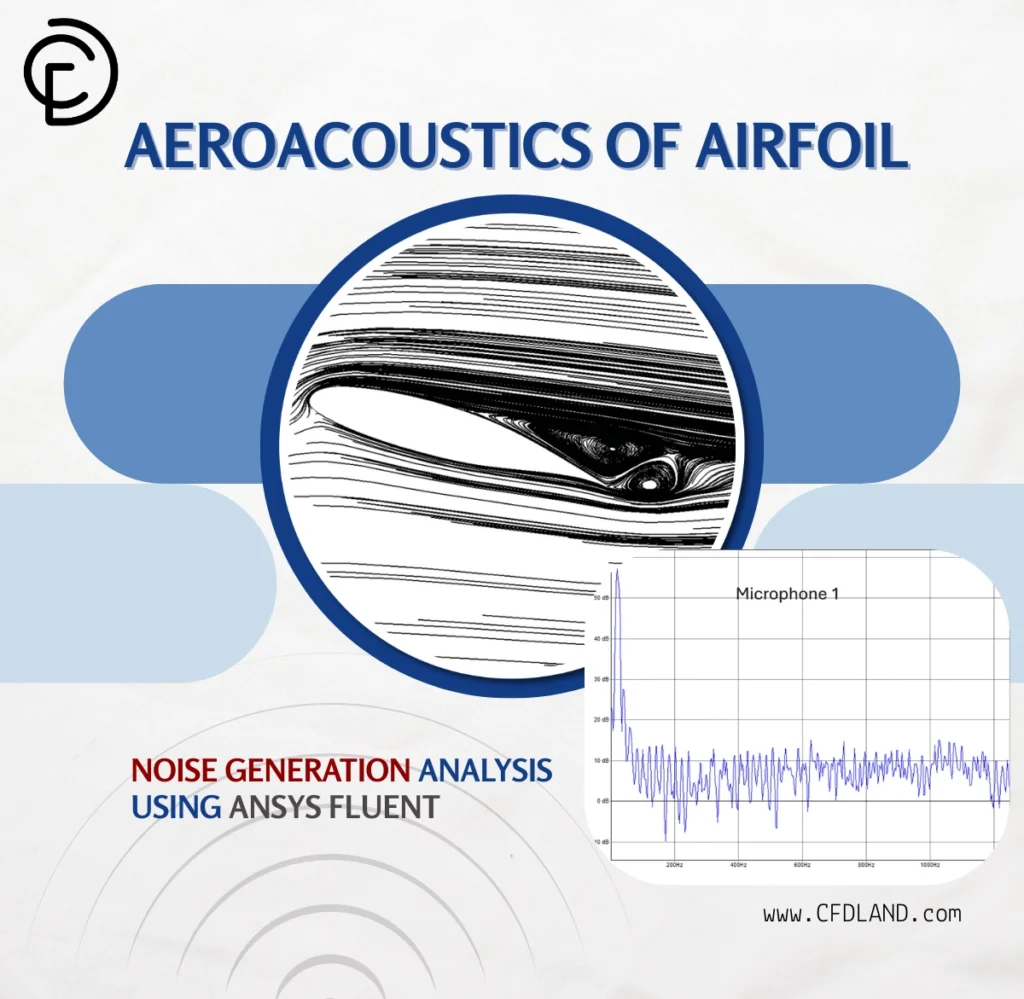
• Aircraft noise: Fast-moving air interacts with airplane wings and engines, creating turbulence and noise. This is a major challenge for engineers working to reduce noise near airports.
• Ventilation systems: When air moves through ducts and interacts with fans, it can cause vibrations and turbulence, leading to unwanted noise in buildings.
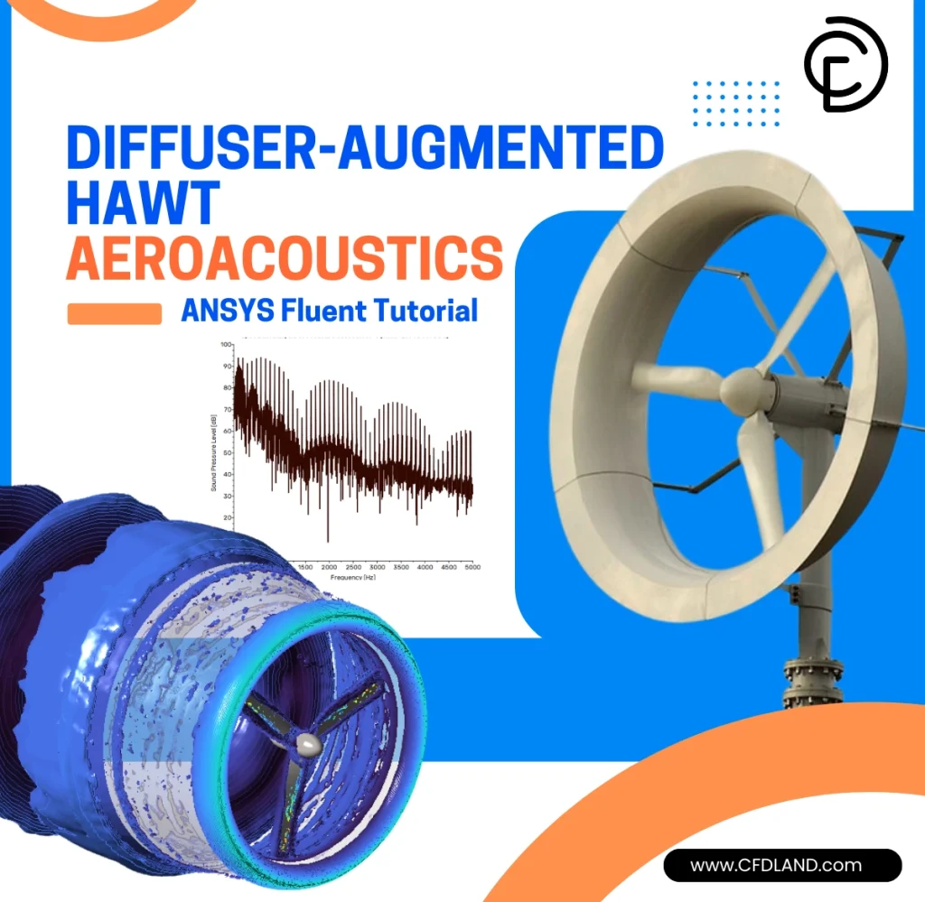
• Wind turbine noise: The spinning blades of wind turbines create airflow patterns that produce sound. Engineers study these flows to design quieter turbines, especially for areas near residential zones.

Another important concept in aeroacoustics is turbulence-induced sound generation. Turbulence occurs when fluid flows become unsteady or chaotic. This happens, for example, when air moves quickly around an object, like the edge of a building or the blades of a fan. Turbulence causes pressure fluctuations—rapid changes in pressure—which produce sound waves that travel through the air. These unsteady flows are often responsible for the loud, roaring sounds of jet engines or the whistling noise of wind passing through narrow gaps.

Figure 3: Engineers study turbulence in fluid flow to understand and reduce aircraft noise

The relationship between fluid dynamics and sound generation is at the heart of aeroacoustics. Engineers use advanced tools, like CFD simulations, to study fluid movement and predict the noise it creates. By understanding how turbulence and pressure fluctuations generate sound, engineers can develop better designs for quieter airplanes, more efficient ventilation systems, and low-noise wind turbines.

Figure 4: CFD simulations help engineers predict how turbulence generates sound.

 

Simulation and Modeling Techniques

Computational Fluid Dynamics (CFD) is a powerful computer-based tool used to study how fluids, like air and water, move. In acoustics, engineers use CFD to understand how sound is created and how it travels. This is very important for aeroacoustics, which is the study of noise generated by airflow. Aeroacoustic simulations help engineers see where noise comes from and how it spreads. This is often difficult to measure with real experiments. By using CFD, engineers can test different designs on a computer to create quieter products and systems.

CFD Methods for Aeroacoustics

To simulate the fluid motion that creates noise, engineers can choose from different CFD methods. Each method has a different level of detail and requires a different amount of computer power.

• Large Eddy Simulation (LES): LES is a detailed CFD method that focuses on the large, swirling structures in a fluid flow, called eddies. These large eddies are often the main source of aerodynamic noise. LES calculates these large structures directly and uses a simpler model for the smaller ones. This gives a good balance between accuracy and computer cost, making it a popular choice for aeroacoustic predictions.
• Direct Numerical Simulation (DNS): DNS is the most accurate CFD method. It calculates all the turbulent motions, from the biggest eddies down to the smallest ones. DNS gives the best possible information about how turbulence creates sound. However, it needs a very powerful computer and a lot of time to run. Because of this, DNS is mostly used for basic research on small and simple problems.
• Reynolds-Averaged Navier-Stokes (RANS): RANS is a simpler CFD method. Instead of calculating the turbulent eddies directly, it uses models to represent their average effect on the flow. RANS is much faster than LES or DNS. It is often used for a first look at an acoustic problem or when computer resources are limited. While it may not capture all the details of noise generation, it provides a good starting point.

Types of Acoustic Modeling in ANSYS Fluent

ANSYS Fluent has several special tools for acoustic simulations. These tools help engineers choose the best way to solve their specific noise problem.

Direct Method is the most complete approach. The simulation directly solves the fluid dynamics equations to calculate both how the sound is made and how it travels. The direct method gives very detailed results, but it is also the most difficult and expensive to run. It is best for studying sound in the near-field, which is the area close to the noise source, like the noise inside a car cabin, whose behavior can be described by the classic Acoustic Wave Equation:

This equation shows how changes in pressure (P) travel outwards as a wave. Because this method captures everything, it is very accurate but also computationally very expensive. It requires extremely fine meshes and small time steps to correctly see both the flow and the tiny pressure waves. In Fluent, there is no single “on/off” button for DAS. It is the result of running a very high-quality transient simulation (like LES or DNS) with a mesh that is fine enough to resolve the acoustic wavelengths. DAS is most practical when the “listener” is very close to the sound source (the near-field), such as when calculating sound pressure inside an airplane or car cabin.

 

Hybrid Acoustic Simulation
The most common and practical approach for engineering problems is Hybrid Acoustic Simulation. This is a two-step process. First, a high-quality CFD simulation is run to calculate the unsteady flow that creates the sound. Second, this flow data is used by a specialized acoustic model to predict how the sound travels. Fluent offers two main hybrid models.

 

Ffowcs Williams-Hawkings (FW-H) Integral Method is a popular tool for predicting noise in the far-field, which is the area far away from the source. This method works by separating the problem into two parts. First, a CFD simulation is run to calculate the fluid flow. Then, the FW-H model uses that flow data on a surface to predict the sound that travels far away. This is much faster than the direct method for predicting far-field noise from objects like airplanes or cars. It is based on an integral equation that separates the complex fluid physics from the sound physics. It works like a set of virtual microphones that listen to the sound created by unsteady pressure on surfaces you choose. To use it, you first run an unsteady CFD simulation (like LES). Then, you activate the model in Fluent by going to Setup > Acoustics > Create/Edit… > Ffowcs Williams and Hawkings…. In this panel, you define the surfaces that are creating noise and the locations of the “receivers” where you want to measure the sound. It is important to know that the standard FW-H model is designed for predicting sound in open space (free-field), like the noise from an airplane wing or a wind turbine. It is not suitable for sound inside an enclosed space, like a pipe. The method is based on an integral equation, which can be conceptually written as:

Where p'(x,t) represents the sound pressure at a specific location and time.

Figure 5: The Ffowcs Williams-Hawkings (FW-H) acoustic method. The flow data on the surface is used to calculate the sound that travels into the far-field.

Wave Equation Approach is a hybrid method. It uses CFD to find where the noise is created. Then, it uses a separate acoustic wave equation to calculate how the sound travels through the area. This approach is very useful for simulations inside enclosed spaces, where sound waves can bounce off walls, such as in an HVAC duct or inside a room, it solves a version of the classic acoustic wave equation to simulate how sound propagates. The general form of the equation is:

Here, ‘S’ represents the source terms, which are calculated from the CFD simulation. This model first uses the CFD results to find the sound sources and then solves the separate wave equation to model the sound propagation. A key advantage of this method is that, unlike FW-H, it is not limited to open-space problems. This makes it very versatile and perfect for modeling sound propagation inside ducts, mufflers, or other enclosures.

Figure 6: The Wave Equation acoustic method in Ansys Fluent.

Some types of noise do not have a single, clear tone. Instead, they sound like a “hiss” or “roar” made of many different frequencies. This is Broadband Noise Source Models, and it is often caused by turbulence. ANSYS Fluent has special models to find where this type of noise is coming from. These models use data from a RANS simulation to show which parts of the flow are creating the most broadband noise. Sometimes, the goal is not to predict the sound at a specific location, but to find out where the noise is coming from. For this, Fluent has Broadband Noise Source Models. These are diagnostic tools used to identify the “hotspots” of sound generation in the flow. Many of these models are based on Proudman’s formula, which links turbulence to acoustic power. The general idea is:

The biggest advantage of these models is that they are computationally very cheap. They can even use the results from a steady-state RANS simulation, which saves a lot of time. This makes them excellent for quick, early-stage design analysis to find the noisiest parts of a design. To use them, you can activate them from the acoustics menu: Setup > Acoustics > Create/Edit… > Broadband Noise Sources…. You can then see the results as contours in your domain to visually identify which areas are generating the most noise.

Figure 7: An example of a broadband noise spectrum predicted using ANSYS Fluent’s source models. This plot shows that the sound energy is spread across a wide range of frequencies.

Method	Primary Goal	Best Application	Required CFD Input	Computational Cost	Key Advantage
Direct (DAS)	Solve for flow and sound simultaneously.	Near-field acoustics, research, where flow & sound are tightly coupled.	High-fidelity Transient (LES/DNS)	Very High	Highest accuracy, captures all physics.
Hybrid: FWH	Predict sound pressure at specific receiver points.	Open-space (free-field) problems like wings, fans, and turbines.	Transient (URANS/LES)	Medium	Very efficient for far-field noise prediction.
Hybrid: Wave Equation	Predict sound pressure and its propagation in a domain.	Enclosed spaces like ducts, mufflers, and cabins where reflections are key.	Transient (URANS/LES)	High	Accurately models sound in complex or enclosed domains.
Broadband Noise Sources	Identify the location of noise sources (“hotspots”).	Early-stage design analysis and quick diagnostic checks.	Steady-State (RANS) or Transient	Very Low	Fast and excellent for pinpointing where noise is being generated.

Using ANSYS Fluent for Acoustic Simulations and Post-Processing

After running a simulation, engineers need to analyze the results to understand the noise. During the simulation, ANSYS Fluent saves the pressure information from each virtual microphone, or “receiver,” into special data files. These files contain the raw pressure signal over time.

To analyze this data, you go to the Results > Reports > Acoustics section in Fluent. Here, you can load the acoustic data file from your simulation. The most important tool for analysis is the Fast Fourier Transform (FFT). The FFT is a mathematical tool that changes the pressure signal from the time domain (how pressure changes over time) into the frequency domain (how much sound energy there is at each frequency). This is like taking a complex musical sound and breaking it down into its individual notes.

When you use the FFT tool, you get a plot of the Sound Pressure Level (SPL). The SPL is measured in decibels (dB) and tells you how loud the sound is at different frequencies. High peaks on this plot show the dominant tones, or the loudest frequencies in the noise. To better match what a person would actually hear, you can apply an A-weighting filter. The human ear hears middle frequencies better than very low or very high ones. The A-weighting adjusts the SPL values to create a result in dBA, which is a better measure of perceived loudness. A great feature is that ANSYS Fluent can also export this data for more advanced analysis or for use in other software.

Figure 8: The post-processing panel in ANSYS Fluent where engineers load acoustic data and use the Fast Fourier Transform (FFT) to calculate the Sound Pressure Level (SPL) spectrum.

Perhaps the most exciting feature is the ability to actually listen to the simulation. ANSYS Fluent can take the predicted pressure signal and convert it into a sound file, like a .wav file. This is incredibly powerful. Instead of just looking at graphs, engineers and designers can directly hear the noise their product will make. Listening to the sound can help identify annoying tones or other noise quality issues that are hard to see on a plot. This feature helps make product design better and faster by providing direct, intuitive feedback.

Applications of CFD in Acoustic Simulation

These advanced simulation techniques are used every day to solve real-world noise problems. On the CFDLAND website, you can find many practical examples of how these models are applied. Let’s look at a few key areas where CFD makes products quieter and better.

Building Aeroacoustics and Wind Noise When strong wind flows around tall buildings, it can create annoying whistling or roaring sounds. To solve this, engineers use a detailed LES simulation to capture the complex, unsteady airflow around the building. Then, they apply the Ffowcs Williams-Hawkings (FW-H) method to predict how that noise travels to nearby areas. The simulation provides important data, such as maps of sound pressure on the building’s walls and plots of the Sound Pressure Level (SPL) at specific locations, like a resident’s balcony. This information is very valuable because it helps engineers see exactly which parts of the building, such as sharp corners or facade elements, are creating the most noise. By analyzing these “hotspots,” they can recommend simple design changes, like rounding the corners, to make the building significantly quieter for its residents.

Figure 9: This simulation shows sound pressure levels on a building’s facade, helping architects identify and fix noisy areas before construction begins.

Figure 10: Data Sound Pressure Level (SPL)

Silencers and Mufflers for HVAC Systems Noise from fans in ventilation systems is a common problem in buildings. A silencer, or muffler, is a device placed in the ductwork to reduce this noise. To design an effective silencer, engineers first use Broadband Noise Source models to simulate the noise created by the fan. Then, they use the Acoustic Wave Model to see how that sound travels through the silencer. The most important output from this simulation is a graph of Transmission Loss (TL), which shows how many decibels of sound the silencer blocks at different frequencies. A good silencer must have a high Transmission Loss at the same frequencies where the fan is loudest. If the simulation shows the performance is poor, engineers can look at sound pressure maps inside the silencer to understand why. This allows them to improve the design, for example by changing the shape or adding more sound-absorbing material, to make it work better.

Figure 11: Sound pressure contours inside a simulated silencer. This analysis helps engineers optimize the internal design for maximum noise reduction.

Turbomachinery Noise from Fans and Engines Fast-spinning blades in fans, pumps, and jet engines create a complex mix of noise. This includes tonal noise, which is a clear hum at specific frequencies, and broadband noise, which is a “whoosh” sound. For a detailed analysis, engineers use LES combined with the FW-H method. The simulation produces SPL plots that clearly show the sharp peaks of tonal noise and the wider curve of broadband noise. It can also create contour plots that show exactly where on the fan blades the noise is being generated. By analyzing the SPL plot, engineers can target specific noise problems. For example, if a specific tone is too loud, they can change the number of blades to move that annoying sound to a less sensitive frequency. If the broadband noise is the problem, they can change the shape of the blades to make the airflow smoother.

Figure 12: A CFD analysis of a cooling fan shows noise sources on the blades. This helps engineers redesign the blade shape to reduce both tonal and broadband noise.

Supersonic Jet Noise The noise from a supersonic jet, like that from a fighter aircraft, is one of the loudest sounds made by technology. To study this, engineers use a very detailed Large Eddy Simulation (LES). LES is needed to accurately capture the two main sources of this intense noise: the violent, turbulent mixing of the high-speed jet with the air around it, and the strong shock waves that form in the flow. The simulation’s output gives a direct visualization of the acoustic pressure fluctuations, which are the sound waves themselves. Engineers can see these waves radiating away from the jet in contour plots. They also get Sound Pressure Level (SPL) data to measure how loud the jet is. This analysis is critical because it allows engineers to see exactly where the loudest noise is being created—whether from the turbulence or the shocks. With this knowledge, they can work on designing new nozzle shapes or control methods to weaken the shock waves and change the turbulent mixing, which helps in developing quieter and more efficient jet engines.

Figure 13: An LES simulation shows acoustic pressure waves (in red and blue) radiating from a supersonic jet. This visualization helps engineers pinpoint the primary sources of jet noise for reduction.

Advanced Wind Turbine Simulation with FSI For some machines, the way the structure moves or vibrates has a big impact on the noise it makes. A great example is a special Gorlov Helical Turbine, which has blades shaped like a screw. To analyze this properly, engineers use a very advanced method called Two-Way Fluid-Structure Interaction (FSI) coupled with an acoustic simulation. This means the computer model calculates two things at the same time: first, how the wind pushes on the turbine blades and makes them bend, and second, how that bending changes the airflow around the blades. After this complex interaction is simulated, the Ffowcs Williams-Hawkings (FW-H) method is used to predict the resulting noise. This complete approach is incredibly powerful because it links the structural safety of the turbine directly to its acoustic performance. Engineers receive data on the stress within the blades to ensure they won’t break, and they also get detailed SPL plots. This helps them design turbine blades that are not only efficient and safe but are also optimized to be as quiet as possible.

Figure 14: A combined FSI and aeroacoustic simulation of a Gorlov Helical Turbine

Combustion Noise and Instabilities Flames inside power plant gas turbines or car engines are not silent; they create a loud roaring sound. Sometimes, the sound waves can feed back into the flame and cause dangerous pressure vibrations called combustion instabilities. To study this, engineers use special CFD models that simulate fluid dynamics, combustion chemistry, and acoustics all together. The key outputs are plots of pressure changing over time inside the combustor and a frequency analysis of that pressure data. Engineers carefully look for very strong, repeating pressure peaks at certain frequencies, as these peaks are a clear sign of a dangerous instability. The simulation helps them understand why the instability is happening, allowing them to change the design, such as the position of the fuel injectors, to make the combustion process stable, safe, and quiet.

Figure 15: Simulating a combustor helps engineers detect pressure instabilities (shown as high-pressure zones) that can lead to damage. The analysis ensures a stable and efficient combustion process.

 

Conclusion – The Future of Acoustic Design

In this article, we have traveled from the basic science of sound to the advanced world of computer simulation. We learned that sound is made of pressure waves and that aeroacoustics is the special study of noise created by moving air. We saw that Computational Fluid Dynamics (CFD) is the most powerful tool engineers have to study, predict, and control this noise. By using methods like LES and models like FW-H in software such as ANSYS Fluent, engineers can now “see” and “hear” the sound a product will make before it is ever built.

The impact of this technology is all around us. The simulations we discussed are helping to solve real-world problems every day. They lead to quieter aircraft engines, more comfortable cars, and more efficient wind turbines that can be placed closer to our communities. By analyzing noise in HVAC systems and industrial machinery, these tools also create quieter buildings and safer workplaces. Being able to test and fix noise problems on a computer saves a lot of time and money, and it leads to better products for everyone.

The future of acoustic design looks even more exciting. Soon, engineers will use Artificial Intelligence (AI) to help them. An AI will be able to test thousands of different designs very quickly to automatically find the quietest possible shape. At the same time, as computers become more powerful, simulations will get even more accurate and faster. We will also see the development of new “smart materials” designed specifically to absorb or cancel sound, and CFD will be essential to understanding how to use them.

The goal of acoustic engineering is simple: to control sound, making our world a better place. As technology advances, the ability to manage noise becomes more important for our health and quality of life. Through the power of simulation, engineers are not just reducing noise; they are designing a quieter, more comfortable, and more peaceful future.