

In our first blog on radiation physics, we learned the fundamental theory of radiation. Now, we will apply that knowledge using the powerful tools inside ANSYS Fluent. Choosing the correct ANSYS radiation model is the most critical step for achieving accurate results in your Radiation CFD simulations. This guide will help you select the best tool for your specific project.
We will provide a simple and clear explanation of each primary model available in ANSYS Fluent, with a special focus on the popular Discrete Ordinates (DO) and Solar Load models. You will learn about:
- The Discrete Ordinates (DO) Model
- The P-1 Model
- The Surface-to-Surface (S2S) Model
- The Rosseland Model
- The Discrete Transfer (DTRM) Model
- The Monte Carlo (MC) Model
- The Solar Load Model
By understanding these options, which are all accessible from the main Radiation Model panel in ANSYS Fluent, you will be able to confidently set up and solve any problem involving radiation heat transfer. For more practical examples, you can explore our hands-on radiation CFD simulation projects.

Figure 1: The main Radiation Model panel in ANSYS Fluent, where you select the best tool for your simulation, from the versatile DO model to the specialized Solar Load model.
Discrete Ordinates (DO) Model
The Discrete Ordinates (DO) model is the most powerful and popular ANSYS radiation model. It is a great choice for nearly any Radiation CFD Simulation. This model works by calculating heat rays from many different directions. This makes it very accurate for all materials, whether they are clear like glass or cloudy like smoke. The main settings for the DO model are in the Angular Discretization panel. This is how you tell Fluent how to look at the heat rays.

Figure 2: The main settings for the DO model in ANSYS Fluent.
- Theta Divisions and Phi Divisions: Imagine you are in a room. You can look up and down, and you can look side to side. Theta (θ) and Phi (φ) are the science words for these directions. These settings tell Fluent how many directions to look from. A higher number gives a more accurate answer but makes the computer work longer. A number of 3 for both is a good start for most projects.

Figure 3: This picture shows the Theta (θ) and Phi (φ) angles for a direction.
- Theta Pixels and Phi Pixels: Pixels are like tiny squares on a screen. This setting adds more small squares to help the computer see the heat rays better, especially near walls. It makes the simulation more accurate without making it much slower.

Figure 4: An illustration of how Theta and Phi Pixels refine the calculation on a surface, increasing the accuracy of the DO model, especially near walls.
The DO model can also do Non-Gray Radiation. This is very important when materials act differently with different “colors” of heat. For example, a window lets sunlight in but keeps inside heat from getting out.
- Number of Bands: This lets you split the heat into different color groups.
- Wavelength Intervals: Here, you set the start and end point for each color group.
We used this in a real project about a solar building with wavelength bands. In that simulation, we needed to see how the glass walls let the sun’s visible light in but trapped the invisible heat inside. We used two bands: one for sunlight and one for heat. This made our Fluent radiation simulation very realistic.

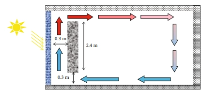
Figure 5: The concept of non-gray radiation, where heat is split into different wavelength bands. This is crucial for accurately simulating materials like glass in solar applications.
The DO model is the best tool for many real-world problems. For example, in our tutorial about solar heat in a room, we used the DO model to see exactly how sunlight from a window warms up the floor and furniture, which then heats the air. In another advanced project, we simulated a parabolic trough solar collector. The DO model was perfect for tracking the sun’s rays as they bounced from a big mirror to a small pipe to heat water. The accuracy of the DO model was essential for that project.


Figure 6: Real-world applications of the DO model, from simulating a parabolic trough solar collector to analyzing how sunlight heats a room in a building.
P-1 Radiation Model
The P-1 model is a simpler and faster ANSYS radiation model. It is a good choice when the material in your simulation is very thick, like smoke or a dense gas. In these materials, heat radiation does not travel very far. The P-1 model is great for these situations because it solves the problem quickly and does not use too much computer power. It is often used in simulations of combustion, glass making, and furnaces.
The main setting for the P-1 model is the Non-Gray Model. This is used when the “color” (wavelength) of heat is important.
- Number of Bands: This lets you split the heat into different color groups. For example, you can tell Fluent to treat sunlight differently from the heat coming from a hot wall.
- Wavelength Intervals: Here, you set the start and end for each color group. You need to tell Fluent the exact wavelength numbers for each band.
Remember, using more bands makes the answer more accurate, but it also makes the computer work much harder. For advanced users, you can also use special codes called User-Defined Functions (UDFs) to control exactly how heat is given off from surfaces.
To understand how powerful the P-1 model is, let’s look at an advanced project. We did a CFD radiation simulation of an ADN monopropellant thruster. This is a modern, “green” rocket engine that uses a special, less toxic fuel. Inside this engine, the fuel burns at extremely high temperatures. This creates a very hot, thick gas. The heat radiation inside this gas is very strong and is a big part of how the engine works. We needed a model that could handle this thick gas but was also fast. The P-1 model was the perfect choice for this Fluent radiation simulation. It helped us see the temperature everywhere inside the engine. This is very important to make sure the engine is safe and works well. This project is a great example of how the P-1 model is used to solve real, complex engineering problems where heat radiation in a thick medium is critical.


Figure 7: A CFD simulation of an ADN monopropellant thruster, where the fast and efficient P-1 model was used to calculate radiation in the optically thick, high-temperature gas.
Surface-to-Surface (S2S) Model
The Surface-to-Surface (S2S) model is a special ANSYS radiation model. It is perfect for problems where heat jumps from one surface to another, and the gas in between does not block the heat. Think of an electric heater in a room. The heat rays travel from the hot heater to the colder walls and furniture. The S2S model is the best choice when the gas (like air) is clear.
This model is different because it does a lot of math before the main simulation starts. It calculates something called View Factors. A view factor is a number that tells you how well one surface can “see” another surface. If two walls are facing each other, they have a large view factor. If they are around a corner, they cannot see each other, so their view factor is zero.
Setting Up the S2S Model
When you choose the S2S model, you will see new settings. The most important one is the View Factors and Clustering box.

Figure 8: Setting up the Surface-to-Surface (S2S) model in ANSYS Fluent. The key step is defining surface clusters and computing view factors to manage computational cost.
Because calculating view factors for every tiny piece of a surface is very slow and uses a lot of computer memory, we use Clustering. This means we group many small faces together into bigger patches. This makes the calculation much faster.
- Faces per Surface Cluster (FPSC): This number tells Fluent how many small faces to put into one big patch. A bigger number means a faster calculation, but it can be a little less accurate. You can set this number yourself (Manual) or let Fluent do it for you (Automatic).
After you set up the clusters, you must calculate the view factors. You have two main choices for the Method:
- Ray Tracing: This is the default method. It works like shooting many tiny laser pointers from one surface. It counts how many lasers hit the other surface to find the view factor.
- Hemicube: This method is like putting a special camera with a wide lens on a surface. It takes a picture to see what other surfaces are visible.
You also need to tell Fluent if surfaces can block each other.
- Blocking: Choose this if some surfaces can be in the way of others. This takes more time but is more accurate for complex shapes.
- Nonblocking: Choose this if there is nothing in the way between the surfaces. This is faster.
Once you have all the settings, you click Compute/Write/Read… to calculate the view factors and save them in a file. This can take a long time. The good news is that you only need to do it once. For future simulations, you can just load the file using the Read Existing File… button.
After the view factors are ready, you can run the simulation. The Iteration Parameters control how the radiation is calculated during the solution.
- Iteration Interval: This tells the computer how often to update the radiation math. A value of 10 is good. It means the computer does 10 steps of its main work, then it updates the radiation.
- Maximum Number of Radiation Iterations: In each radiation update, the computer tries to get the answer right. This number tells it how many times to try. The default of 5 is usually enough.
- Residual Convergence Criteria: This is a small number that tells the computer when the radiation answer is “good enough” and it can stop trying for that step.
Real-World Examples with the S2S Model
The S2S model is very useful for specific engineering problems. In our tutorial on Automotive Paint Curing, we simulated a car part in a big oven. The oven walls were very hot. The heat radiation jumped from the hot walls directly to the car part to dry the paint. The air inside the oven was clear and did not block the heat. The S2S radiation model was the perfect choice for this because it accurately calculated the heat exchange only between the surfaces.
Another great example is our project on Heat Transfer in a Cavity. We looked at a simple square box with one hot wall and one cold wall. The heat radiation jumped from the hot wall to the cold wall. The S2S model was the right tool because we only cared about the heat exchange between the surfaces, not the air in the middle.
Finally, in our simulation of a heater in a room, the hot heater surface gives off heat rays. These rays travel through the clear air and hit the walls, floor, and furniture, warming them up. The S2S model helped us see exactly which surfaces got warmer because of the heater’s radiation.


Figure 9: Practical applications of the S2S model, perfect for problems like automotive paint curing and heat transfer in a cavity, where radiation occurs between surfaces in a clear medium.
Rosseland Model
The Rosseland model is a simple and very fast ANSYS radiation model. It is used for a very special and important situation: when a material is “optically thick”.
What does “optically thick” mean? It means the material is so dense or cloudy that you cannot see through it. Think about very thick, dark smoke, hot melted glass, or even the inside of a star. In these materials, heat rays cannot travel far. They get absorbed and re-emitted almost immediately.
The Rosseland model is fast because it uses a smart trick. It treats the complex movement of radiation inside these thick materials as a much simpler process, like heat moving through a solid metal block (conduction). This makes the math very easy for the computer.

Figure 10: Molten glass is a perfect example of an optically thick medium, where the simple and fast Rosseland model is the ideal choice for radiation analysis.
This model is named after Svein Rosseland, a pioneering astrophysicist from Norway. He was one of the first great scientists in theoretical astrophysics. He developed this model to understand how heat moves deep inside stars, which are very optically thick. His work helped us understand the physics of stars, and now engineers use his ideas to solve problems on Earth.
A great industrial example is making glass. The furnace is full of melted glass that is extremely hot and thick. It is optically thick. For a CFD radiation modeling analysis of this furnace, the Rosseland model is the perfect choice. It helps engineers quickly and accurately understand the temperature inside the thick liquid glass, which is very important for making good quality products.

Figure 11: Norwegian astrophysicist Svein Rosseland, whose pioneering work on heat transfer inside stars gave us the efficient Rosseland radiation model used in engineering today.
Important Note: You should only use the Rosseland model for these thick materials. It is not correct for clear gases like air, or for empty space. It is also less accurate near the boundaries where the thick material touches a wall. But for the right problem, it is a very powerful and fast tool in Fluent radiation simulation.
Discrete Transfer (DTRM) Model
The Discrete Transfer (DTRM) model is another ANSYS radiation model. It works in a very clever way. It shoots rays of heat out from the walls and surfaces of your model. It then follows these rays to see where they go, which cells they pass through, and where they end up. This model is a good choice for many general problems.
The most important part of the DTRM is the “ray file”. Before you start the main simulation, Fluent does a special calculation. It traces all the heat rays and saves a map of their paths into this special file. This can take some time, but you only have to do it once. During the main simulation, Fluent just reads this map instead of calculating the paths again and again. This saves a lot of time.
When you select the DTRM, a new window called the DTRM Rays dialog box will open automatically. This is where you set up the map for the heat rays.

Figure 12: The DTRM Rays dialog box, where you control the number of surface clusters and heat rays to create an efficient “ray file” map for the simulation.
In this window, you need to set up two main things:
- Controlling the Clusters: To make the calculation faster, we group many small faces on the walls into bigger patches. This is called clustering.
- Faces Per Surface Cluster: This number tells Fluent how many small faces to group into one big patch. A bigger number makes the first calculation faster.
- Controlling the Rays: From each big patch (cluster), Fluent shoots out heat rays.
- Theta Divisions and Phi Divisions: These numbers tell Fluent how many rays to shoot out from each patch and in what directions. Think of it like a flashlight. More rays give a more accurate answer but take longer to calculate for the ray file.
After you set these numbers and click OK, Fluent will calculate the ray map and save it to the “ray file”. It is very important to remember that if you change your model in any way—for example, if you change the shape or make the mesh finer—you must create a new ray file.
Monte Carlo (MC) Model
The Monte Carlo (MC) model is a very powerful and accurate ANSYS radiation model. It works differently from all the others. It does a simulation inside your simulation. It works by tracking many thousands of tiny packets of heat energy called “photons”.
Imagine you have a hot wall. The MC model shoots out thousands of tiny virtual photons from this wall. It then follows each single photon on its journey. It watches to see what happens:
- Does the photon hit another wall?
- Does it get absorbed by the gas?
- Does it bounce off (scatter) in a new direction?
The computer records the full life story, or “history,” of every single photon. By tracking millions of these photon histories, the model builds a very accurate picture of how heat is moving in your simulation.
The settings for the MC model let you control the accuracy and speed of this process.

Figure 13: Setting up the highly accurate Monte Carlo (MC) radiation model. The ‘Target Number of Histories’ is the key parameter for balancing precision with simulation time.
- Target Number of Histories: This is the most important setting. It tells Fluent how many photon life stories to track. The default is 100,000. If you use a small number, your results might look “speckled” or noisy, like a bad photo. If you want a smooth and accurate answer, you must use a very high number. More histories give a better answer but make the computer work much longer.
- Mesh Options: You can use the Target Cells Per Volume Cluster to group small cells together. This can make the radiation calculation faster, but it might reduce accuracy a little bit.
- Non-Gray Model: The MC model is also great for non-gray radiation. You can set the Number of Bands to look at different “colors” of heat. For each band, you set the start and end wavelength.
The Monte Carlo model is excellent for very complex problems. For example, if you are simulating a fire with lots of thick, swirling soot, the MC model is a great choice. It can accurately track how the heat photons bounce off the soot particles. This makes it a very powerful tool for difficult CFD radiation modeling problems.
Solar Load Model
This is a special model in ANSYS Fluent made just for one thing: the sun. When you need to simulate the heating effect of sunlight on a car, inside a building, or on a solar panel, this is the perfect tool. The best feature of this model is the Solar Calculator. You do not need to look up the sun’s position. You just tell Fluent the location on Earth (latitude and longitude), the date, and the time of day. Fluent will automatically calculate the sun’s exact direction and strength for you.

Figure 14: The main settings for the Solar Load Model, with the powerful Solar Calculator open. You can input the time, date, and location to automatically find the sun.
The Solar Load Model gives you two main options:
- Solar Ray Tracing: This is the most common option. It shoots sun rays into your model from the calculated sun direction. It is very smart and can figure out which surfaces are in the sun and which are in the shade. It then adds the sun’s heat directly to the surfaces that are hit by the rays. It is a very fast and practical way to see how the sun heats up an object.
- Solar Irradiation: This option is a helper for the DO or MC models. It does not calculate the heat by itself. Instead, it tells the DO or MC model where the sun is and how strong the sunlight is. The DO or MC model then does the full radiation calculation, including the sunlight.
The Solar Load Model is very powerful for renewable energy and building design. We have used it in many CFD radiation modeling projects. For example, we can simulate:
- How a solar chimney uses the sun’s heat to create a natural airflow for ventilation.
- How much heat gets trapped inside a glass greenhouse, which is important for growing plants.
- The best design for a flat-plate solar collectorto capture the most energy for heating water.
- How a 3D solar stilluses sunlight to evaporate and purify water.
- The performance of a hybrid PV/T collector, which generates both electricity and hot water from sunlight.


Figure 15: Solar ray tracing application from CFDLAND shop
Conclusion
We have explored all major ANSYS radiation models in Fluent radiation simulations. Each model serves a specific purpose:
- DO Model: Most versatile, handles complex problems with participating media
- P-1 Model: Fast and simple for diffuse radiation
- S2S Model: Perfect for surface-to-surface radiation in clear media
- Rosseland Model: Fastest option for optically thick materials
- DTRM Model: Good general-purpose ray tracing method
- MC Model: Highest accuracy but computationally expensive
- Solar Load Model: Specialized tool for simulating sunlight effects
Choosing the right model depends on your optical thickness, geometry complexity, and computational resources. For most CFD radiation modeling problems, start with the DO model. For clear media with surface radiation, use S2S. For solar applications, the Solar Load model with its built-in solar calculator is invaluable.