Conjugate Heat Transfer (CHT)

Conjugate Heat Transfer (CHT) represents a critical aspect of modern engineering design, where understanding the interaction between solid and fluid domains is essential for developing efficient thermal systems. As discussed in our article on Overall Heat Transfer Coefficient, accurate prediction of heat transfer rates requires consideration of multiple heat transfer mechanisms simultaneously. This comprehensive guide explores the fundamentals, applications, and simulation techniques of CHT using ANSYS Fluent.

What is Conjugate Heat Transfer (CHT)?

Conjugate Heat Transfer refers to the coupled thermal interaction between solid and fluid domains where heat transfer occurs simultaneously through different mechanisms. As explained in our article on Convective Heat Transfer, this process involves the continuous heat flux and temperature at solid-fluid interfaces, making it essential for accurate thermal analysis.

Table 1. Solid, Fluid, and Interface heat transfer Characteristics

Domain	Primary Heat Transfer Mechanism	Characteristics
Solids	Conduction	Heat transfer through material structure
Fluids	Convection	Heat transfer through fluid motion
Interface	Combined	Continuous temperature and heat flux

 

Conjugate Heat Transfer Examples and Applications

CHT analysis finds applications across various industries, particularly in thermal management and energy systems such as in heat sinks, battery systems, cooling systems, heaters, PV systems, etc. Here are two notable examples from our CFD SHOP:

1. Nanofluid (Single-phase) in Microchannel Heat Sink CFD Simulation, ANSYS Fluent Training: This advanced simulation demonstrates how nanofluids enhance microchannel heat sink performance. The system achieves a thermal resistance of 0.011698232 K/W, showing significant improvement over traditional cooling methods. The simulation involves complex geometry modeling and structured grid generation using ANSYS Meshing software.

Figure 1: Conjugate Heat transfer in  Microchannel Heat Sink CFD Simulation, ANSYS Fluent Training

  2. Photovoltaic Thermal System (PVT) Using DO Radiation Model CFD Simulation: This innovative system combines photovoltaic and thermal technologies for simultaneous electricity and heat generation. The simulation validates system performance with only a 3.07% difference from experimental results, demonstrating the accuracy of CHT analysis in renewable energy applications.

Figure 2: Conjugate heat transfer in Photovoltaic Thermal System (PVT) CFD Simulation

Photovoltaic Thermal systems (PVT) combine photovoltaic and solar thermal technologies to produce electricity and heat concurrently from one system. These systems usually include solar panels that capture sunlight and convert it into electricity. They also use the panels’ heat to produce hot water or space heating. Through integrating these two technologies, PVT systems provide enhanced energy efficiency and maximize the utilization of solar resources. This makes them a highly appealing choice for generating renewable energy in residential and commercial settings. With the integration of photovoltaic and thermal capabilities, the energy output of solar energy systems is maximized, resulting in improved overall performance.

Conjugate Heat Transfer Theory

The theoretical foundation of CHT involves solving coupled equations for solid and fluid domains simultaneously. In solids, heat transfer primarily occurs through conduction, governed by Fourier’s Law:

Where:

K is thermal conductivity, rho is density, Cp is specific heat capacity, T is temperature and t is time.

For fluids, as discussed in our article on the Energy Conservation Equation, the heat transfer equation includes additional terms for convection and energy transport:

Where:

v is fluid velocity and S represents source terms.

At solid-fluid interfaces, the following conditions must be satisfied:

1. Temperature continuity
2. Heat flux conservation
3. No-slip condition for viscous fluids

Different Ways Heat Can Transfer in Solid and Fluid

Heat transfer in engineering systems occurs through three fundamental mechanisms that work together in complex thermal systems. Understanding these mechanisms is crucial for effective thermal system design and analysis. Let’s explore each mechanism in detail with its governing principles and practical applications.

Conduction Heat Transfer

Conduction represents the primary mechanism of heat transfer in solid materials, occurring through molecular interactions within the material structure. This process involves the transfer of kinetic energy between adjacent molecules, where energy moves from higher temperature regions to lower temperature regions without bulk material movement.

The fundamental equation governing conduction heat transfer is expressed through Fourier’s Law:

In three dimensions, this expands to:

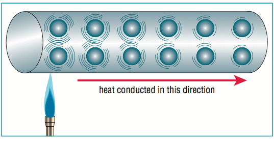
Figure 3: Conduction Heat Transfer – adopted from https://superakbov.best/product_details/75825923.html

Figure 3 illustrates the conduction process through a solid material. The image shows a clear temperature gradient from the hot side (red) to the cold side (blue), with arrows indicating the direction of heat flow. The molecular vibrations within the material are represented by interconnected particles, demonstrating how thermal energy transfers through the solid structure. This visualization helps understand how conduction occurs at the molecular level while showing the macroscopic temperature distribution.

Convection Heat Transfer

Convection involves heat transfer through fluid motion and represents the dominant heat transfer mechanism in fluids. This process combines the effects of conduction within the fluid and energy transport through bulk fluid movement. The basic mathematical expression for convective heat transfer is Newton’s Law of Cooling:

For forced convection analysis, we often use the dimensionless Nusselt number correlation:

Figure 4: Convection Heat Transfer adopted from https://chemicalengineeringworld.com/modes-of-heat-transfer/

Figure 4 provides a comprehensive visualization of both natural and forced convection processes. The image shows fluid flow patterns around a heated surface, with arrows indicating fluid movement. Natural convection is illustrated by rising hot air currents, while forced convection is shown through mechanically driven flow patterns. The color gradients effectively demonstrate temperature variations within the fluid.

Radiation Heat Transfer

Radiation represents a unique heat transfer mechanism that occurs through electromagnetic wave propagation, requiring no physical medium for energy transfer. The Stefan-Boltzmann Law governs radiation heat transfer:

For radiation exchange between surfaces:

Figure 5: Radiation Heat Transfer – adopted from https://www.flaticon.com/free-icon/sun-radiation-symbol_34531

Figure 5 depicts radiation heat transfer through electromagnetic waves. The illustration shows wavy arrows representing radiation emanating from a hot surface and being absorbed by cooler surfaces. This visualization helps understand how thermal energy can transfer through space without a medium, particularly relevant in solar radiation and high-temperature applications.

Combined Heat Transfer Effects

Figure 6 presents a comprehensive view of all three heat transfer mechanisms operating simultaneously in a practical application. The illustration shows how conduction occurs through solid walls, convection takes place in surrounding fluids, and radiation exchanges heat between surfaces at different temperatures. This integrated visualization helps understand how these mechanisms work together in real-world scenarios.

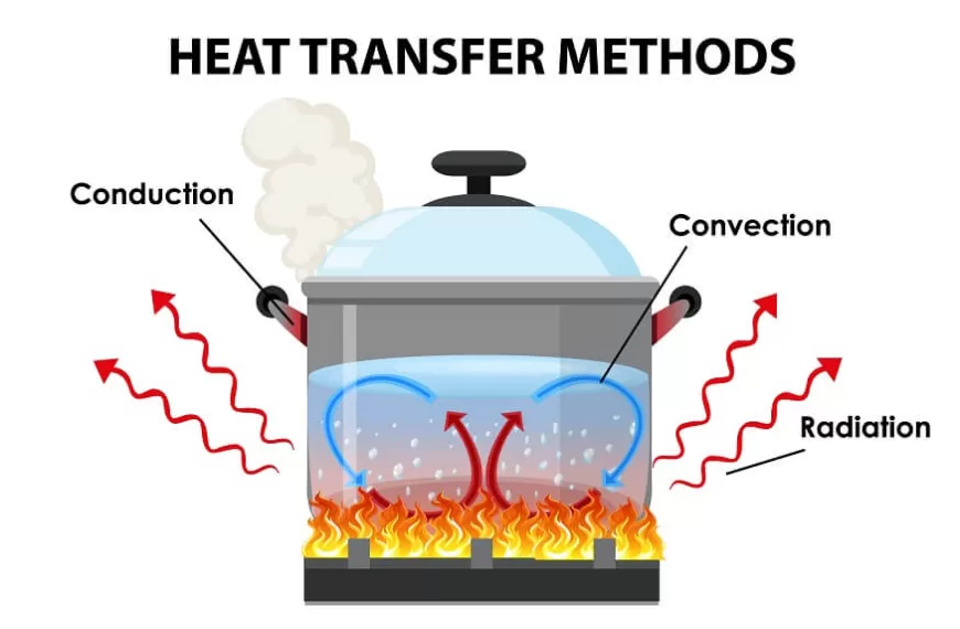
Figure 6: Combined Heat Transfer Mechanisms – adopted from https://www.eurokidsindia.com/blog/heat-transfer-methods-for-kids.php

Summary Table of Heat Transfer Methods

Table 2 provides a crucial overview of how each mechanism operates in different domains:

Table 2. Transfer Methods in Fluid and Solid Domains

Transfer Method	Solid Domain	Fluid Domain	Primary Equation
Conduction	Primary mechanism	Secondary mechanism
Convection	Not applicable	Primary mechanism
Radiation	Surface phenomenon	Participating medium

 

This comprehensive understanding of heat transfer mechanisms forms the foundation for conjugate heat transfer analysis in engineering applications. In practical applications, these mechanisms rarely operate in isolation, and their combined effects must be considered for accurate thermal system design and optimization.

Geometry and Mesh Generation

The foundation of any successful simulation begins with creating an accurate geometry of the system. This process involves defining both solid and fluid domains while ensuring proper interface representation between them. The geometry must accurately represent the physical system being modeled, including all relevant features that could affect heat transfer and fluid flow.

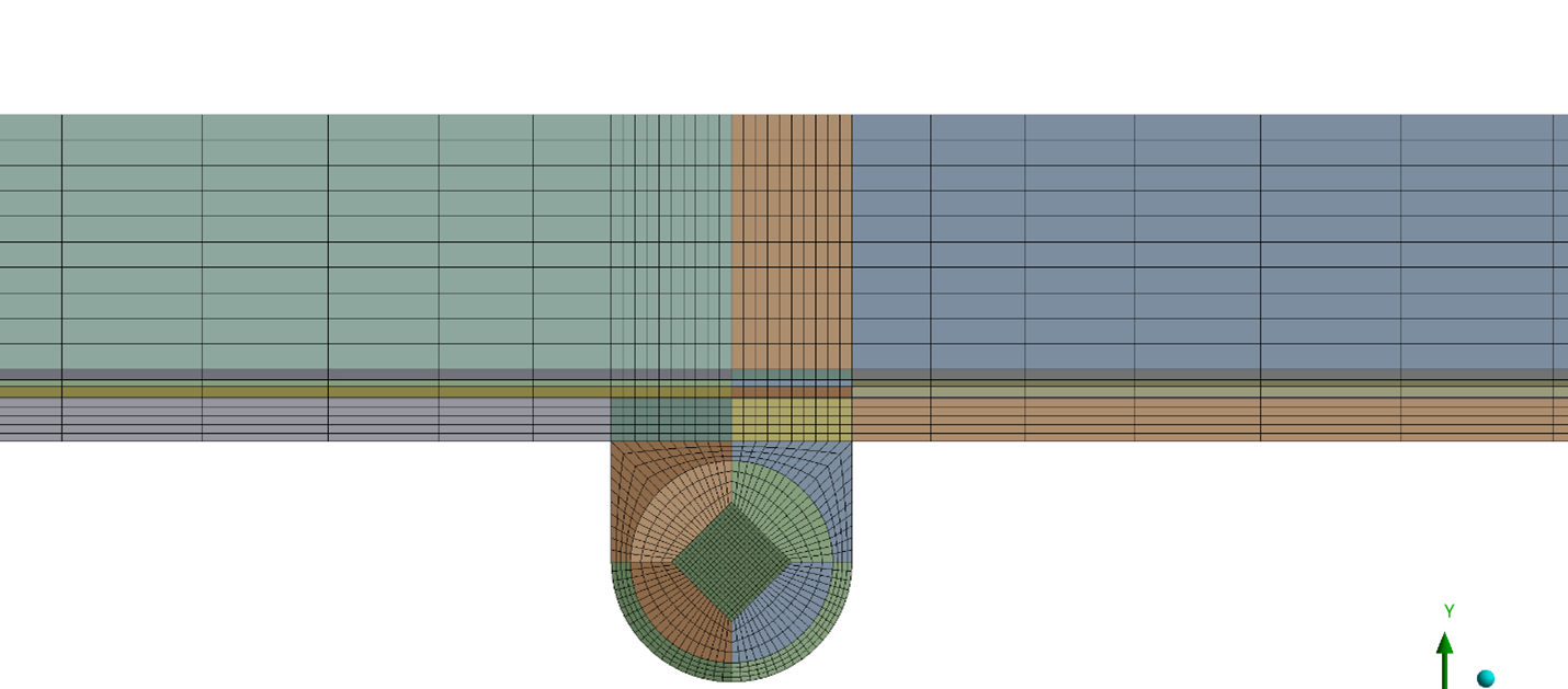
Figure 7: Elements generated for the solid and fluid domains

Once the geometry is established, the next crucial step is mesh generation. Figure 7 demonstrates the elements generated for both solid and fluid domains. The mesh quality shown in the figure reveals different element sizes and distributions, particularly refined near critical regions such as interfaces and boundary layers. The mesh density must be carefully balanced – fine enough to capture detailed thermal gradients and flow patterns, yet optimized to maintain reasonable computational costs. The figure clearly shows how elements transition between regions, ensuring proper connectivity and numerical stability.

Material Property Definition

Material properties form the cornerstone of accurate thermal analysis. Figure 8 presents the ANSYS Fluent materials window, where users can define and modify material properties for both solid and fluid domains. This interface allows engineers to specify crucial properties such as thermal conductivity, density, specific heat capacity, and viscosity. The figure demonstrates the comprehensive material database available in ANSYS Fluent, along with options to create custom materials and implement temperature-dependent properties.

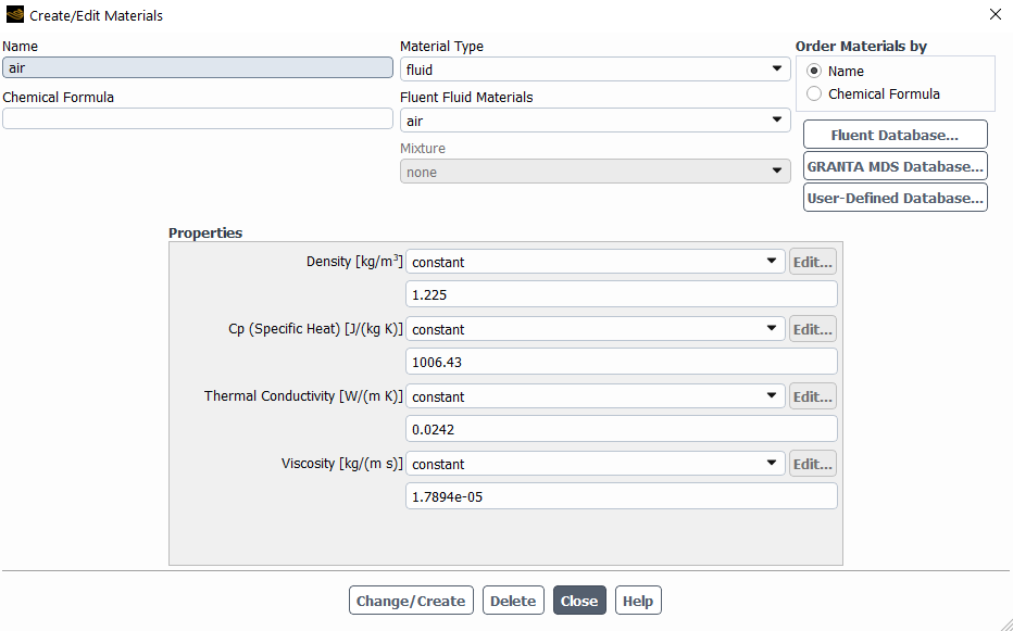
Figure 8: Materials window in ANSYS Fluent to specify properties for a CHT simulation

Boundary Condition Specification

Boundary conditions define the physical constraints and operating conditions of the thermal system. Figure 9 illustrates the interface boundary condition window, showing the various options available for specifying thermal and flow conditions at domain boundaries. The figure highlights how engineers can define temperature profiles, heat flux distributions, and interface coupling parameters. These conditions must accurately represent the real-world operating environment, including temperature or heat flux at solid-fluid interfaces, fluid inlet and outlet conditions, and external heat sources or sinks.

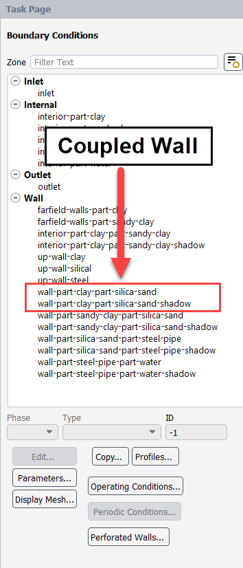
Figure 9: Coupled wall boundaries in CHT simulation using ANSYS Fluent

Solution Method Selection

The selection of appropriate solution methods significantly impacts simulation accuracy and convergence. Figure 10 displays the cell zones configuration interface, where users can choose solver settings, turbulence models, and numerical schemes. This window allows engineers to define solution parameters based on the specific requirements of their simulation, whether dealing with laminar or turbulent flows, steady-state or transient conditions.

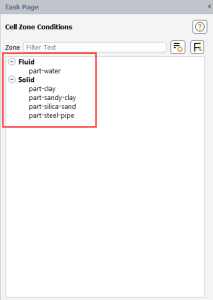
Figure 10: Cell zone condition in ANSYS Fluent

Solution and Post-Processing

The final stage involves solving the simulation and analyzing results through post-processing tools. The additional Figure 5 showing the Photovoltaic System provides an excellent example of post-processing capabilities. This visualization demonstrates temperature distributions, flow patterns, and heat transfer characteristics across the system. Engineers can use these visualizations to identify critical areas of thermal stress, evaluate system performance, and optimize design parameters.

Through these comprehensive steps and proper utilization of ANSYS Fluent’s capabilities, engineers can effectively analyze and optimize thermal systems across various applications. The software’s robust features, combined with proper understanding of conjugate heat transfer principles, enable the development of efficient and reliable thermal solutions.

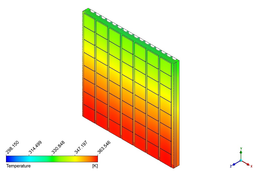
Figure 11: Visual sample in case of the Photovoltaic System

Conclusion

Conjugate Heat Transfer analysis is fundamental for modern thermal system design and optimization. Through ANSYS Fluent’s capabilities, engineers can accurately simulate complex heat transfer phenomena across solid-fluid interfaces. Understanding and implementing CHT is crucial for developing efficient thermal solutions across various industries.

For practical implementation and detailed tutorials, explore our CFD Shop, including the microchannel heat sink and PVT system simulations mentioned above.