DPM Breakup Models: Droplet Disintegration Physics & Setup

Understanding droplet breakup during Discrete Phase Model (DPM) CFD simulations is basic for accurately capturing spray and atomization phenomena. In this comprehensive guide, we will explore the physics of droplet disintegration. We will practically discuss the six DPM breakup models provided in ANSYS Fluent. By understanding the underlying physics such as the two-body direct breakup model under the long-wavelength approximation, you can optimize industrial applications like fuel injection, mist spray systems, and agricultural spraying.

DPM Breakup Concepts: Atomization Regimes

Generally, the atomization regimes can be categorized into two main stages:

Primary Breakup (Jet Breakup)

This stage consists of three regimes:

1. Rayleigh jet
2. First wind-induced
3. Second wind-induced

These regimes describe the continuous disintegration of a liquid jet as it pinches off from a nozzle. The Rayleigh jet regime, as illustrated in Figure 1, shows the initial stages of jet breakup. In this stage, surface tension forces dominate the aerodynamic forces (such as drag – read our DPM Drag Law Models guide for more info). As a result, the liquid jet breaks into large, distinct droplets.

However, this early stage will soon be substituted by wind-induced regimes because the aerodynamic forces take the lead. This transmission results in a more chaotic and unorganized breakup pattern. As time goes by, the atomization regime transitions into the secondary breakup process.

Figure 1: Atomization regimes in primary breakup – [Reference: Analysis of diesel spray atomization by means of a near-nozzle field visualization technique]

Secondary breakup (Droplet breakup)

Extra forces are needed to destroy the central sheet, ligaments, and separated droplets to transition from primary breakup to the secondary stage. Hydraulic instabilities and body forces, such as acceleration, are the keys to a fully developed spray.

The Weber number (We) plays a leading role in determining this breakup behavior. This dimensionless parameter represents the ratio of deforming inertial forces to cohesive forces:

$$\text{We} = \frac{\rho u^2 L}{\sigma}$$

• We = Weber number
• ρ = fluid density
• u = velocity of the fluid
• L = characteristic length (e.g., diameter of a droplet or jet)
• σ = surface tension of the fluid

A higher Weber number means lower surface tension or higher aerodynamic forces. In other words, the higher the Weber number, the faster the transmission from the Rayleigh jet regime to complete atomization.

DPM Breakup Models in ANSYS Fluent

In ANSYS Fluent, six specific breakup models are provided: TAB, Wave, KHRT, SSD, Madabhushi, and Schmehl. You must first enable breakup in the physical models panel alongside Unsteady Particle Tracking. Then, in the Set Injection panel ==> Physical Models tab, you can see the Breakup sub-section (see Fig. 2). (If you want to read more about these sub-models, check our DPM Physical Models Tab Blog).

 

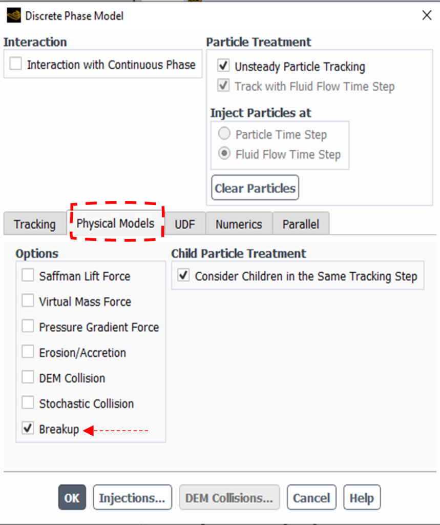
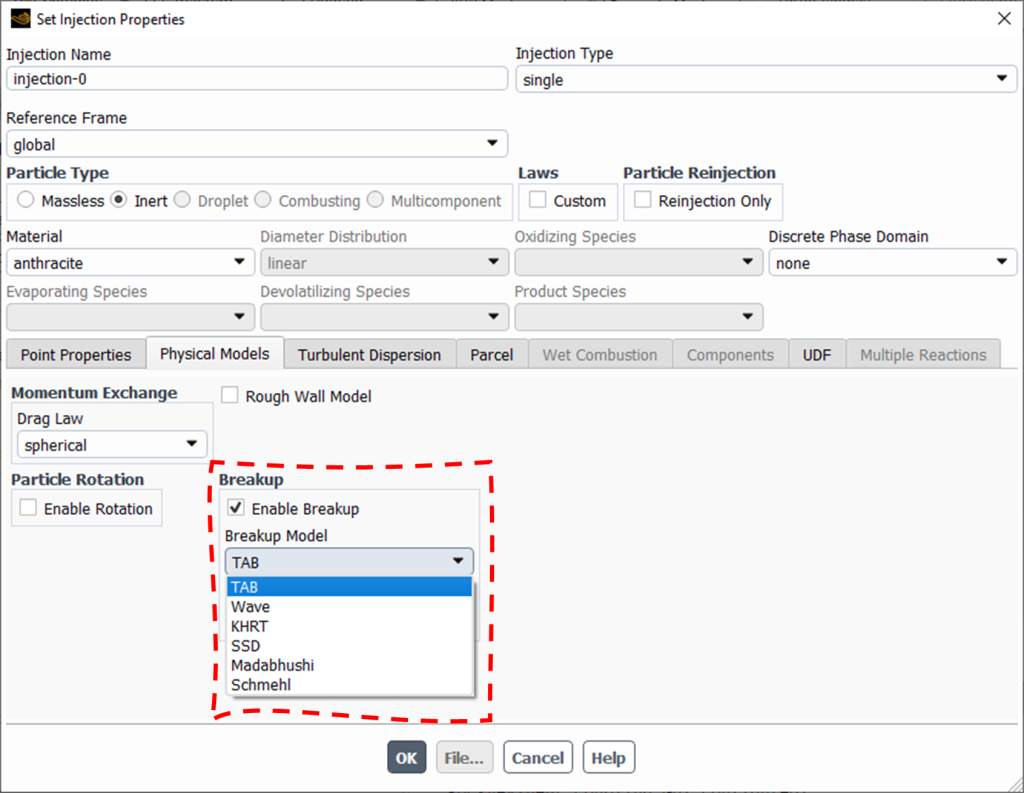
Figure 2: DPM breakup models in ANSYS Fluent: step 1: enable breakup sub-model – step2: find breakup models in injection box

Note: Each DPM breakup model has a complex theoretical background found in the ANSYS Theory Guide. This article adopts a practical approach, focusing on pivotal application information and necessary fundamentals.

1) TAB Breakup Model (Taylor Analogy Breakup)

The Taylor Analogy Breakup (TAB) model, as its name suggests, relies on Taylor’s analogy between an oscillating droplet and a spring-mass system to predict droplet behavior. It is mostly applicable in evaporating spray systems and low-speed sprays (We < 100).

Generally, in the TAB model, the spring-mass system relates to a distorting and oscillating droplet through the following analogous components:

• Restoring force of spring ==> Surface tension forces
• External force ==> Droplet drag force
• Damping force ==> Droplet viscosity forces

This analogy once again proves the importance of knowing drag laws in DPM concepts. Avoiding complex governing equations, the droplet breakup in this model occurs when the distortion exceeds a critical ratio of the droplet radius, typically set at:

$$ x > C_b r $$

Where:

• x is the horizontal distortion of the droplet from a spherical state
• Cb is the constant value equal to 0.5
• r is the spherical droplet radius

To employ the TAB breakup model in ANSYS Fluent, the software asks you to specify two factors (see Fig. 3):

1. Y0: Represents the initial distortion at time zero. Increasing Y0 means faster breakup ==> Smaller droplet diameter ==> Shorter penetration length (due to drag force).
2. Breakup Parcels: This parameter represents the sum of parent and child parcels during a breakup event.

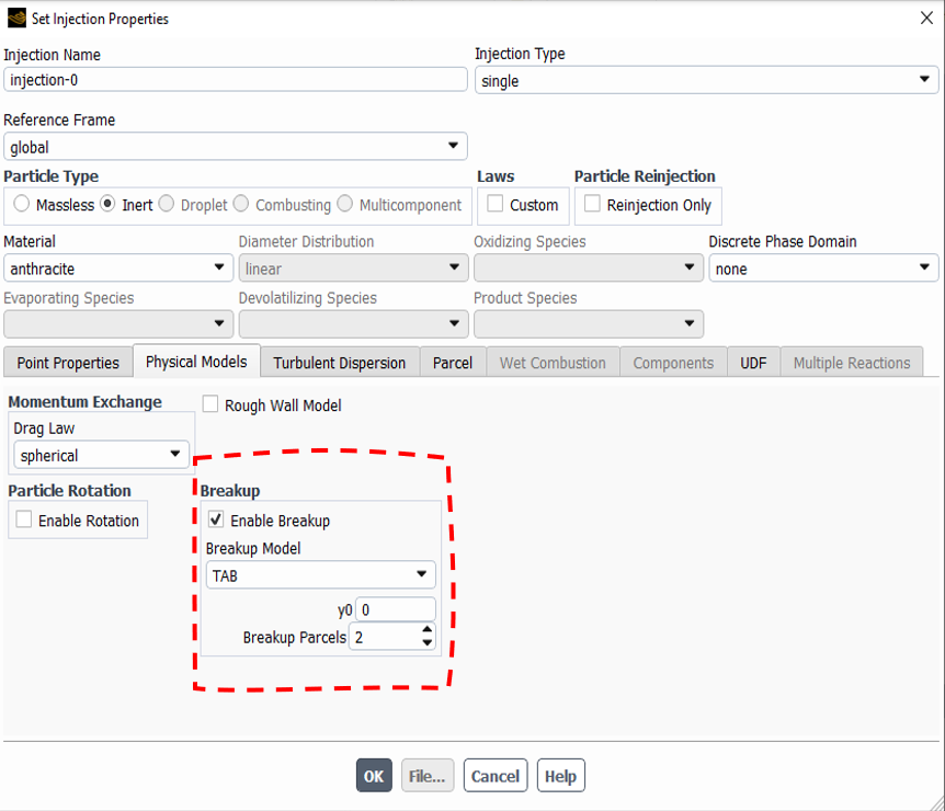
Figure 3: TAB breakup model in ANSYS Fluent

For instance, Figure 4 illustrates a scenario where 3 parcels are injected. If the Breakup Parcel parameter is set to 4, each parent parcel produces 3 child parcels, resulting in a total of 12 parcels (3 parents, and 9 children).

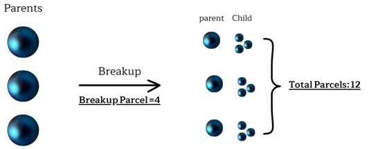
Figure 4: Parent and Child parcels after breakup under TAB model

2) Wave Breakup Model

The Wave Breakup Model, developed by Reitz, is a wise choice for simulating droplet breakup in high-Weber-number flows (We > 100). Inaccurately described in some references as just an alternative to the TAB model, the Wave breakup model fundamentally assumes that droplet breakup is induced by the relative velocity between gas and liquid phases.

At its core, the Wave model employs a mathematical formulation based on the Kelvin-Helmholtz instability theory. This is closely related to the physics found in the two-body direct breakup model under the long-wavelength approximation, ensuring accurate calculation of droplet fragmentation based on instability wavelengths. The model accumulates mass from the parent drop at a rate given by:

$$\frac{dm}{dt} = -\frac{m_p – m_s}{\tau}$$

Where:

• m_p is the mass of the parent drop
• m_s is the mass of the stable drop size
• τ is the breakup time

This process continues until the shed mass equals 5% of the initial parcel mass, at which point a new parcel is created. Then, the radius of the new droplet is determined by:

$$r = B_0 \Lambda$$

Where:

• B_0 is a model constant (typically 0.61, default in ANSYS Fluent)
• Λ represents the wavelength of the fastest-growing instability on the liquid surface

Now, let’s check the parameters ANSYS asks the user to define when using the Wave breakup model (see Fig. 5).

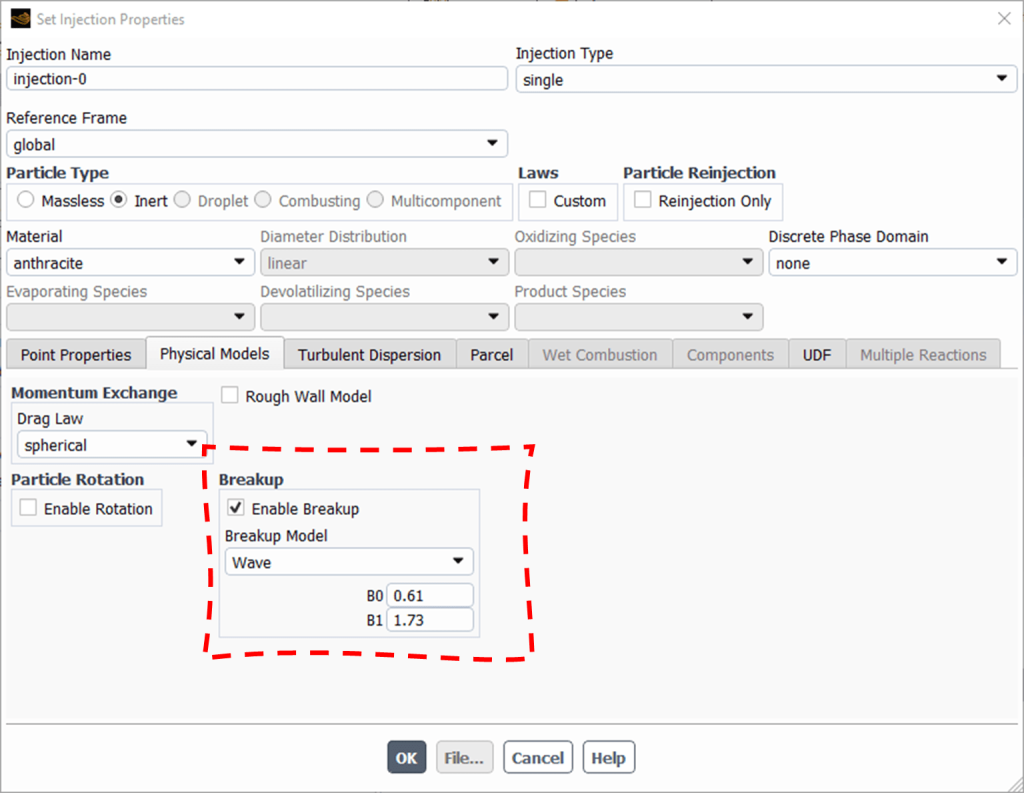
Figure 5: B0 & B1 parameters in Wave Breakup Model in ANSYS Fluent

• B_0 (usually 0.61): Influences drop size.
• B_1: The breakup time constant, determining mass loss rate.

Tip: A larger B_1 value means slower mass loss and less intense gas-liquid interaction. According to the ANSYS guide, it is recommended to be between 15-60.

Tip: Larger B_1 ==> Larger droplet size ==> Longer Penetration Length.

3) Kelvin-Helmholtz / Rayleigh-Taylor (KHRT) Breakup Model

The KHRT (Kelvin-Helmholtz Rayleigh-Taylor) Breakup Model, as its name says, combines two distinct physical mechanisms to predict droplet breakup:

• Kelvin-Helmholtz waves driven by aerodynamic forces
• Rayleigh-Taylor instabilities due to the acceleration of shed drops

This model tracks wave growth on the droplet surface like the Wave breakup model, with breakup occurring due to the fastest-growing instability based on local conditions.

The KHRT model assumes the liquid core is near the nozzle region, and child droplets are shed from the liquid core because of abrupt acceleration during injection to the freestream. The liquid core approximation follows a concept called “blobs” which you can read more about in references, see Fig. 6.  The length of this core is calculated using the following equation:

$$L = C_L \cdot d_0 \sqrt{\frac{\rho_l}{\rho_g}}$$

Where:

• L is the liquid core length
• CL is the Levich constant
• d0 is a reference nozzle diameter
• ρl and ρg are the liquid and gas densities, respectively

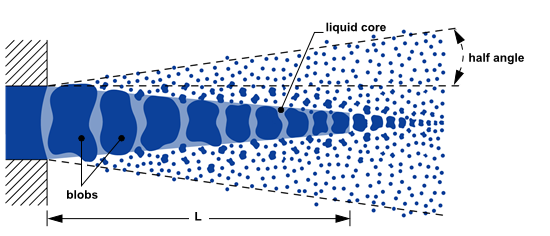
Figure 6: KHRT model and liquid core near nozzle region with blobs approximation – adopted from ANSYS Help

So the question is when to use KHRT model?

Knowing the fundamentals makes it understandable. The KHRT model is handy for simulating high-Weber-number and high-pressure sprays. Based on the literature, the KHRT model can be employed where Catastrophic Breakup is expected (see Fig. 7).

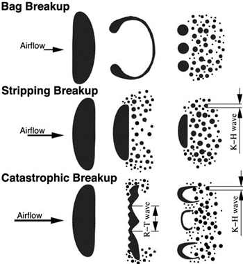
Figure 7: KHRT breakup model and catastrophic breakup – [Reference: Handbook of Atomization and Sprays]

To put the KHRT breakup model into use in ANSYS Fluent, the software asks you to specify five parameters (Fig. 8). These are divided into two categories:

Wave (KH) Model Constants:

• B0: Default value of 0.61. It influences the initial conditions of the liquid jet and its stability.
• B1: Recommended range is 15-60. A larger B1 value will delay the Kelvin-Helmholtz (KH) breakup, allowing users to control the timing of the primary breakup process.

RT Model Constants:

• CL: The Levich model constant. A larger CL value indicates a longer breakup length.
• Ctau: The breakup time constant. It determines how fast the breakup process occurs.
• CRT: Determines the criteria and time required for Rayleigh-Taylor (RT) breakup. A smaller CRT value makes the RT breakup process faster and produces smaller droplets.

Figure 8: KHRT breakup model in ANSYS fluent

Tip: The KHRT model results in a lower penetration length compared to the wave breakup model.

4) Stochastic Secondary Droplet (SSD) Breakup Model

The SSD model is utilized for high Weber number sprays under diesel and gas turbine conditions.

Unlike models that use a single-diameter scale, the SSD model treats droplet breakup as a discrete random event. To some extent, this approach brings an uneven distribution of diameter scales over a range, resulting in a more realistic simulation. Moreover, breakup probability is not dependent on parent droplet size in the SSD breakup model. The secondary droplet size is sampled from an analytical solution (the Fokker-Planck equation).

Governing Equations: It is essential to comprehend the following governing equations to utilize the SSD model properly:

$$r_c = \frac{We_{cr} \cdot \sigma_l}{\rho_g \cdot u_{rel}^2}$$

Where:

• Wecr is the critical Weber number
• σl is the surface tension
• ρg is the gas density
• urel is the relative velocity

and also:

$$t_{bu} = B \cdot \sqrt{\frac{\rho_l}{\rho_g} \cdot \frac{r}{|u_{rel}|}}$$

Where:

• B is the breakup constant
• ρl is the liquid density
• r is the droplet radius

Tip: The breakup applies to droplets larger than the critical radius (Step 1). When a droplet’s breakup time exceeds the critical breakup time, a breakup occurs (Step 2).

Now look at Fig. 9 to see the ANSYS inputs for the SSD breakup model:

• Critical We: Default value is 6.
• Core B1: Defines the breakup time (default 1.73).
• Xi: A negative dimensionless parameter determining how much smaller child particles are than the original parcel.
• Target NP: Controls the number of parcels created during a breakup event.

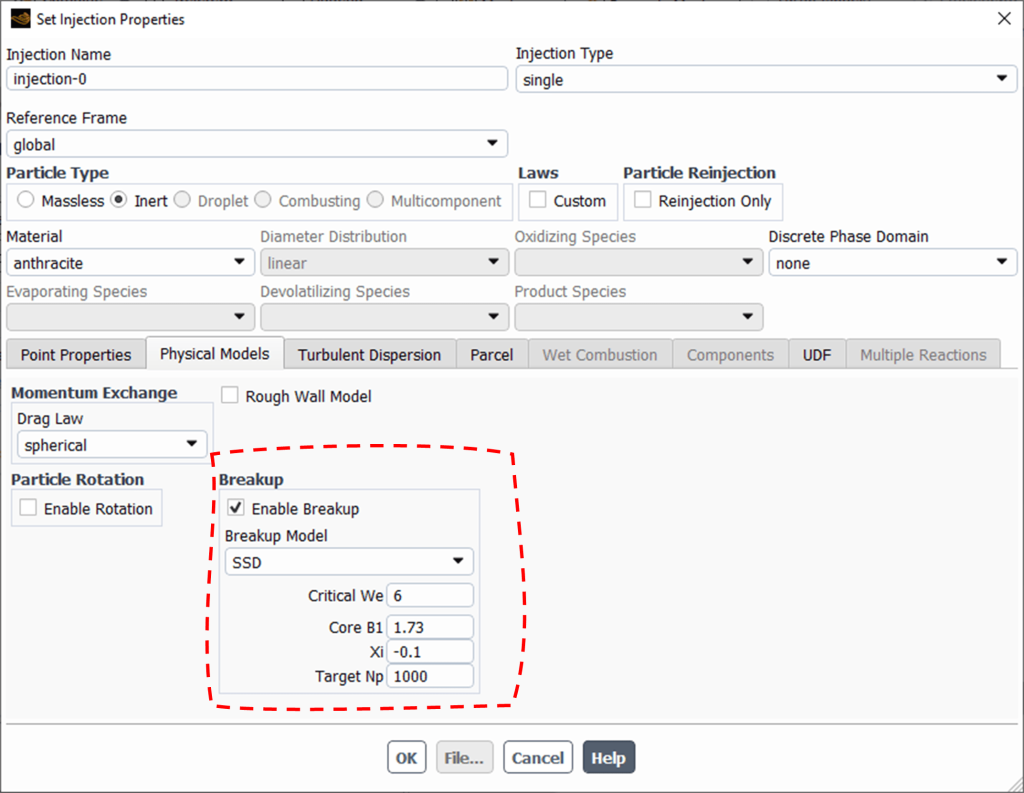
Figure 9: SSD breakup model parameters in ANSYS Fluent

5) Madabhushi Breakup Model

As discussed earlier, when a liquid is injected into a gas, it typically undergoes Primary Breakup and Secondary Breakup. The Madabhushi breakup model addresses the drawbacks of traditional methods:

• Primary Breakup: It uses the Wave breakup model to simulate the initial breakup of the liquid column.
• Secondary Breakup: This is where Madabhushi differentiates itself. It considers the formation of ligaments (irregularly shaped fragments breaking off the liquid core), which represents a highly realistic real-world scenario (See Fig. 10).

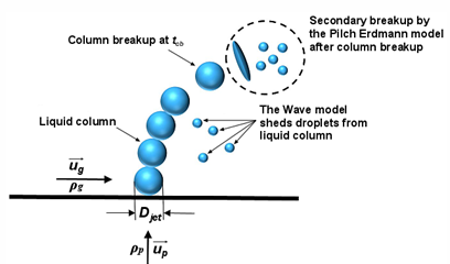
Figure 10: Madabhushi breakup model – Reference: ANSYS Help

Tip: As stated, the Madabhushi model considers the formation of ligaments. Madabhushi introduces a weighting factor for accounting the impact of ligaments on child droplet sizes.

To implement the Madabhushi breakup model in ANSYS (Fig. 11), we must define:

• B0: Affects initial breakup behavior (0.61 default).
• B1: Influences the secondary breakup process (1.73 default).
• C0: Column breakup time constant (1.44 default).
• Column Drag Cd: Drag coefficient during column breakup (1.48 default).
• Ligament Factor: Directly affects child droplet size forming in secondary breakup (0.4 default).
• Jet Diameter [m]: The nozzle orifice exit diameter.
• Breakup Max Generation: Limits the number of generations of droplet breakup to prevent excessive computational load.
• Subsequent Statistical Breakup: When enabled, this activates a statistical model after reaching the Max Generation limit, adjusting particle diameters while maintaining total mass.

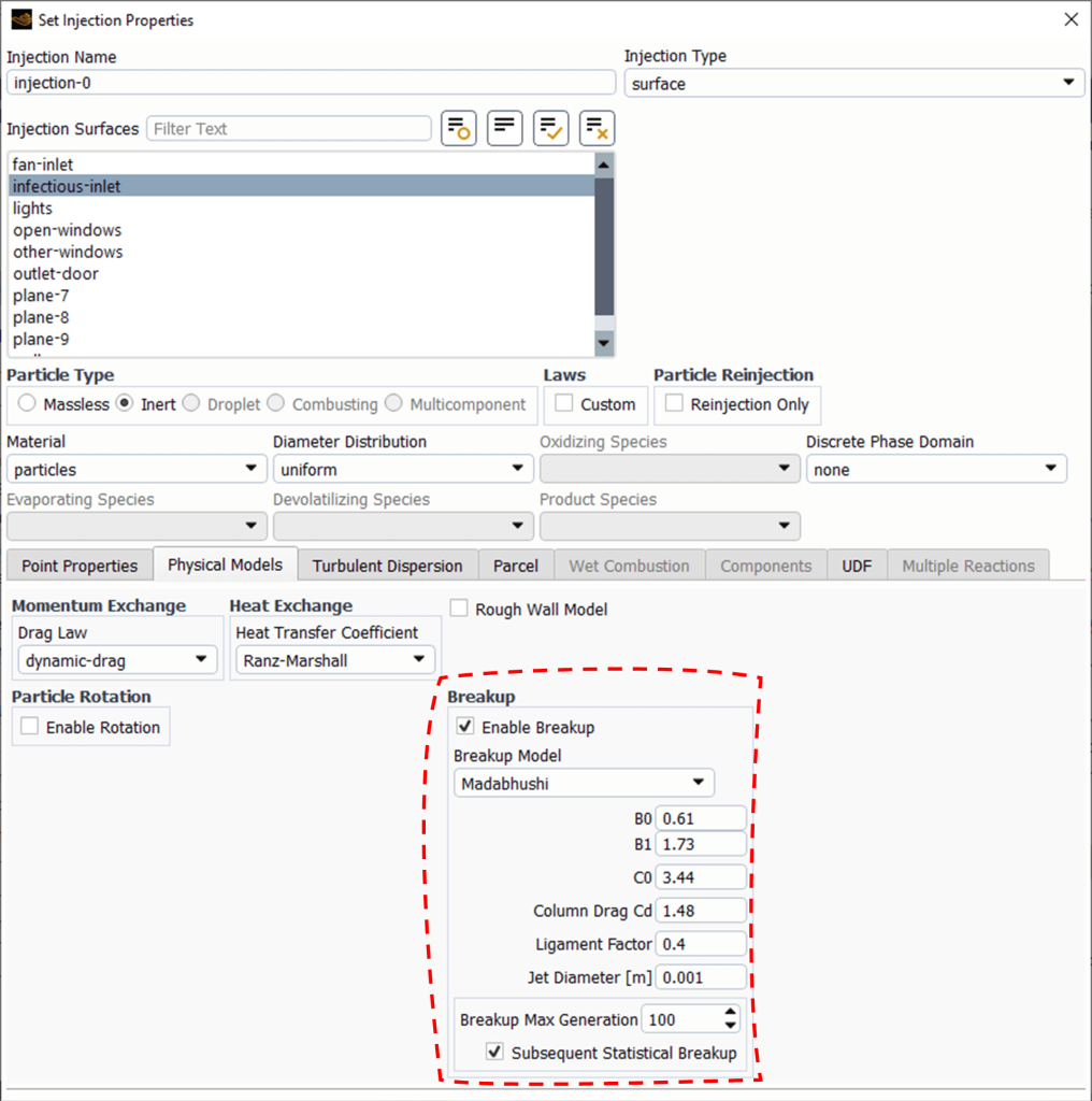
Figure 11: Madabhushi breakup model in ANSYS Fluent

6) Schmehl Breakup Model

The Schmehl breakup model distinguishes breakup regimes into three distinct categories based on the Weber number (We) and Ohnesorge number (Oh):

• Bag Breakup
• Multimode Breakup
• Shear Breakup

The Ohnesorge number assesses the damping effect of viscous friction against surface tension within the droplet:

Weber number is introduced in the introduction of the blog. The Ohnesorge number assesses the damping effect of viscous friction against surface tension within the droplet:

$$Oh = \frac{\mu}{\sqrt{\rho \sigma D}}$$

Where μ is the dynamic viscosity.

The Schmehl model switches between these regimes considering local Weber numbers:

• Deformation with no breakup: We≤Wecrit=12(1+1.077Oh1.6)
• Bag Breakup: Wecrit<We≤Wemultimode=20(1+1.2000Oh1.5)
• Multimode Breakup: Wemultimode<We≤Weshear=32(1+1.5000Oh1.4)
• Shear Breakup: Weshear<We

Tip: Regardless of the regime, the Schmehl model divides the breakup process into two stages: initial deformation into a disc shape, followed by disintegration. In Bag Breakup and Multimode Breakup regimes, the volumetric distribution of child droplets follows a root-normal distribution:

This two-stage approach allows for an understanding of how different forces interact to cause droplet breakup.

Tip: The behavior of child droplets formed during breakup varies across the different regimes:

In Bag Breakup and Multimode Breakup regimes, the volumetric distribution of child droplets follows a root-normal distribution, similar to the Madabhushi model:

$$f(x) = \frac{1}{\sqrt{2\pi}\sigma} e^{-\frac{(x-\mu)^2}{2\sigma^2}}$$

However, in the Shear Breakup regime, the distribution is bimodal. Approximately 80% of the parent droplet’s mass forms small droplets due to shear forces, while the remaining 20% forms larger core droplets.

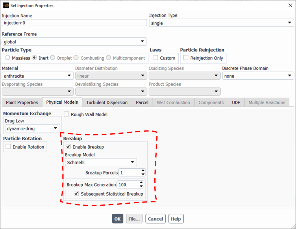
Figure 12: Schmehl breakup model in ANSYS Fluent

Conclusion and Next Steps

Choosing the right atomization model whether you rely on the Wave model, the KHRT model, or the advanced physics of the two-body direct breakup model is crucial for your CFD accuracy. We hope this guide provided a clear understanding of the six DPM breakup models available in ANSYS Fluent.

If you need professional assistance implementing these models for multiphase flows, explore our DPM CFD Simulation Tutorials Category. Additionally, if you require a tailored solution for your project, you can Order Your CFD Project.