

The DPM window in ANSYS Fluent consists of different sections. As shown in Fig. 1, there is a separate tab named Physical Models. This tab provides various options for tracking each particle in a Lagrangian framework. Before investigating these options in-depth, we should briefly mention the governing equation. The CFD solver predicts the particle trajectory by integrating the force balance acting on it. This balance is written in a Lagrangian reference frame and equates the particle’s inertia with the surrounding forces. For example, the motion in the x-direction in Cartesian coordinates is:
[latexpage]
\[
\frac{du_p}{dt} = F_D(u – u_p) + \frac{g_x(\rho_p – \rho)}{\rho_p} + F_x
\]
Where:
• The first term on the right side is the drag force per unit particle mass.
• The second term accounts for gravity and buoyancy forces.
• Fx represents additional forces that become important under special circumstances.
The options inside the Physical Models tab mainly focus on defining these additional forces (Fx). Given this introduction, we can now investigate each option provided in the software.
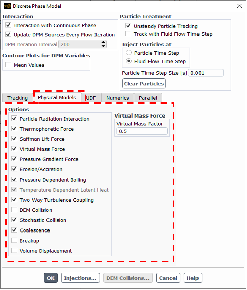
Figure 1: Discrete Phase Model (DPM) panel in ANSYS Fluent
Particle Radiation Interaction
The Particle Radiation Interaction model is valuable in applications where radiation plays a prominent role in thermal processes, such as in combustion chambers. When you activate this model, the software calculates the radiative heat transfer to and from the particles. This interaction influences the temperature of both the discrete and continuous phases, affecting the overall flow dynamics.
Note: This option is available only if you have already activated the P1 or Discrete Ordinates (DO) radiation model.
What`s more, you must specify two extra radiative properties for the particle materials: Particle emissivity and scattering factor (see Fig. 2).
Particle emissivity defines the particle’s ability to emit radiation. It is a dimensionless number from 0 to 1, where 1 means a perfect emitter (blackbody). Generally, emissivity is 1 for coal, 0.5 for ash, and about 0.95 for water droplets.
Similarly, the scattering factor defines how much incident radiation the particle scatters. This is also a dimensionless number between 0 and 1. A value of 0 means no scattering, while 1 means total scattering. This factor highly depends on particle size. As a general rule, use 0 for soot particles and 0.5 to 1 for water droplets.
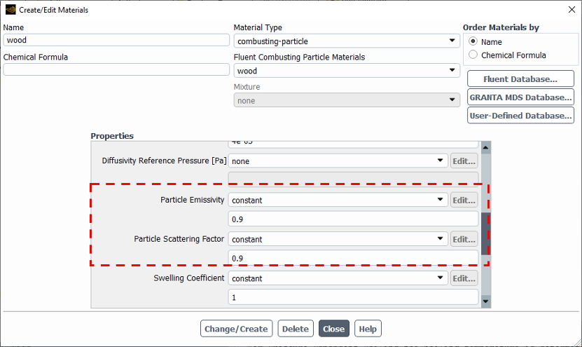
Figure 2: Particle emissivity and Particle scattering factor in the particle material properties section of ANSYS Fluent
Thermophoretic Force
The Thermophoretic Force refers to the force exerted on particles due to a temperature gradient in the surrounding fluid. Physically, this force happens because of the difference in momentum transfer between gas molecules and the particles. Molecules on the hotter side have more kinetic energy. Therefore, they impart more momentum to the particle and push it toward the cooler side. You should always include this additional force in problems with high temperature gradients.
Mathematically, this additional force (Ft) is defined as:
F_t = -C_t \mu d_p^2 \frac{\nabla T}{T}
Where:
• Ft: Thermophoretic force
• Ct: A constant (typically around 1.17)
• μ: Dynamic viscosity of the fluid
• dp: Particle diameter
• ∇T: Temperature gradient
• T: Absolute temperature of the fluid
As seen in Fig. 3, the software uses the Talbot-diffusion model to predict the thermophoretic coefficient. This model uses particle size and gas properties to provide a more accurate description of the force.
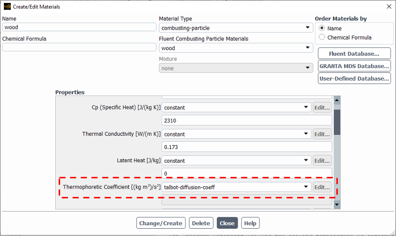
Figure 3: Thermophoretic coefficient model in ANSYS Fluent
Saffman Lift Force
The Saffman Lift Force acts on particles moving through a fluid when a velocity gradient (shear) exists in the surrounding flow. Under this condition, the particle experiences a lift force perpendicular to the flow direction. We will not cover the mathematical formulation here. However, the most important point is that the Saffman lift force is significant only for small particles (micron range and below). It becomes negligible for larger particles because forces like drag dominate the flow.
Virtual Mass Force and Pressure Gradient Force
You must activate the Virtual Mass Force and Pressure Gradient Force to improve particle dispersion predictions in cases where the density of the continuous phase is greater than or equal to the density of the discrete phase (e.g., bubbles dispersed in a liquid).
Scientifically, the virtual mass force appears when a particle accelerates within a fluid. It accounts for the additional inertia the fluid exerts on the particle. The virtual mass factor determines the intensity of this force. A value of 1 applies the standard force, values above 1 increase the effect, and values below 1 reduce it (see Fig. 4). Likewise, if the density ratio is above 1, you must consider pressure gradient effects by activating the Pressure Gradient Force option.
Density of continuous phase >= Density of Discrete phase
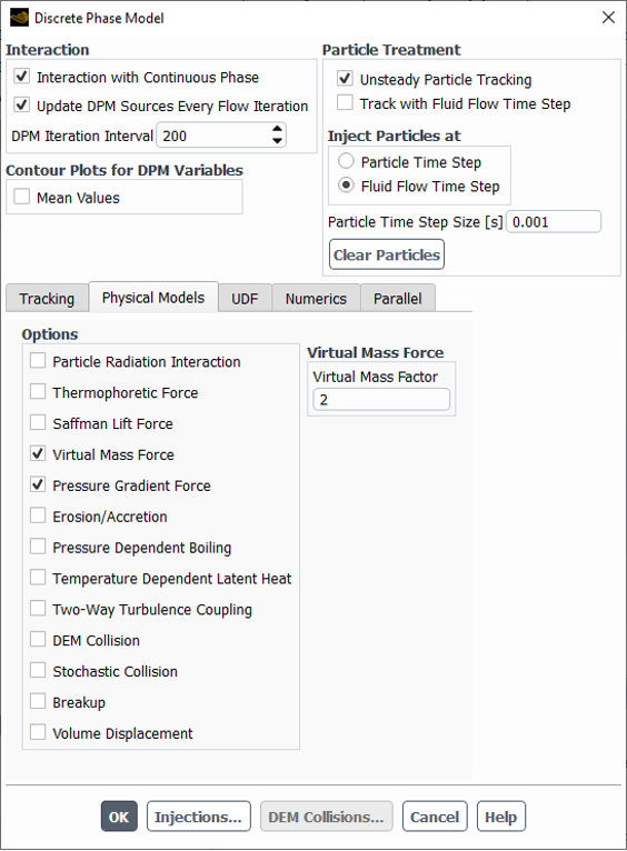
Figure 4: Virtual mass factor in DPM panel
Particle-Wall Erosion & Breakup Models
The Physical Models tab also includes options for droplet fragmentation (Breakup) and particle-wall damage (Erosion/Accretion). Because these topics involve vast theories, complex mathematical formulations, and dedicated sub-models (such as TAB and Wave for breakup, or Finnie and Oka for erosion), we do not cover them here to avoid redundancy.
- For particle-wall damage, please read our ultimate guide to erosion modeling.
- For aerodynamic droplet fragmentation, please refer to our dedicated DPM Breakup Models blog.
Pressure Dependent Boiling
The boiling point of a liquid is the temperature at which its vapor pressure equals the surrounding pressure. Pressure-dependent boiling refers to the phenomenon where this boiling point varies as domain pressure changes. As pressure increases, the boiling point increases, and vice versa.
In simulations where the pressure deviates from atmospheric levels, it is essential to adjust the boiling point. Enabling this option allows the solver to automatically switch from droplet vaporization (Law 2) to droplet boiling (Law 3) based on local conditions.
By default, the solver transitions from vaporization to boiling when the particle reaches a predefined, static boiling point. However, with this option enabled, the transition condition changes. The software now compares the saturation vapor pressure at the droplet temperature against the domain pressure (Psat>P). If the domain pressure exceeds the saturation vapor pressure, the model correctly reverts to the vaporization law.
You must provide accurate droplet saturation vapor pressure data that covers the entire temperature and pressure range of your simulation. Lastly, when this option is active, the Temperature-Dependent Latent Heat model is applied automatically.
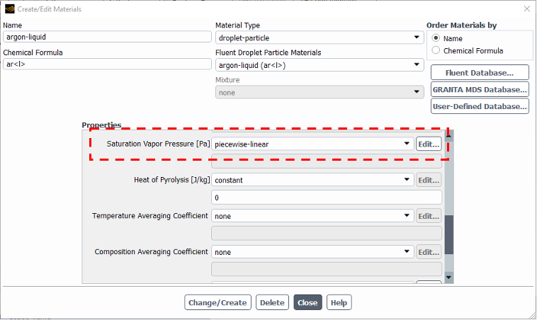
Figure 6: saturation vapor pressure when using Pressure dependent boiling model
Two-way Turbulence Coupling
In cases where the dispersed phase affects the turbulence of the continuous fluid, the Two-way turbulence coupling option leads to a more realistic approach. This option calculates the changes in turbulent quantities caused by particle damping and the generation of turbulence eddies.
DEM Collision
DEM Collision refers to Discrete Element Method modeling. This approach simulates the mechanical behavior of granular materials. If your flow features a high volume fraction of the dispersed phase, DEM collision is crucial because high concentration leads to continuous particle-particle interactions.
In CFD theory, this approach is known as 4-way DPM coupling. It includes:
1. Continuous phase effect on Discrete Phase
2. Discrete phase effect on Continuous phase
3. Discrete phase effect on itself (particle-particle interaction)
Activating this model opens further panels to describe collision partners and contact force laws (see Fig. 7).
Note: For highly advanced particulate flows, the ANSYS Rocky extension specializes in simulating granular materials and provides deeper DEM capabilities.
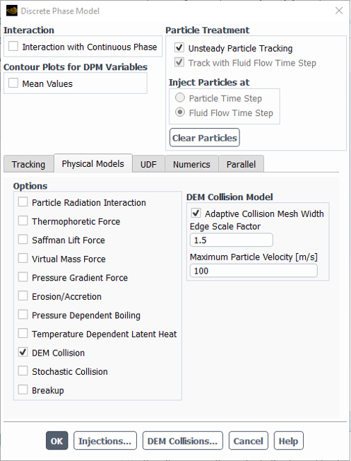
Figure 7: DEM Collision in Discrete Phase Model Physical Models of ANSYS Fluent
Stochastic Collision and Coalescence
Due to the extremely high computational cost of the DEM collision model, the software offers a practical alternative. Stochastic Collision and Coalescence is a simpler, highly efficient method for handling particle interactions. Instead of simulating detailed mechanics for every particle, it relies on statistical models and averages.
The coalescence sub-model becomes available only if you activate stochastic collision. Coalescence is the process where two or more particles merge to form a single larger particle upon collision. This is particularly relevant in systems where droplet growth is important, such as spray nozzles or emulsion flows.
Technically, after two particles collide, the algorithm determines the outcome. For liquid droplets, it considers both coalescence and bouncing. For solid particles, only bouncing occurs. The probability of these outcomes depends on the collisional Weber number (We), which characterizes the ratio of inertial forces to surface tension forces:
[latexpage]
\[
We = \frac{\rho u^2 L}{\sigma}
\]
ρ = Density of the fluid (kg/m³)
u = Characteristic velocity of the fluid (m/s)
L = Characteristic length (typically the diameter of the droplet or particle) (m)
σ = Surface tension of the fluid (N/m)
Important Tip: This model is best suited for low-Weber-number collisions (We<100). Also, if your particle time step is excessively large, it will influence and corrupt the statistical results. Always adjust the particle length scale appropriately.
Volume Displacement
Volume Displacement refers to the effect that discrete particles have on the continuous phase by physically occupying space within the fluid domain. When particles take up a significant volume, they displace the fluid, creating a phenomenon known as the blockage effect.
While this effect is often negligible in highly dilute flows, it becomes critical in dense systems. You can set the maximum particle volume fraction used to compute the blockage via the software’s text user interface (TUI) command:
define/models/dpm/interaction> max-vf-allowed-for-blocking
The standard recommended value for the maximum DPM volume fraction in continuous flow is 0.95.
Properly configuring the Physical Models tab ensures your simulation matches real-world physics, whether you are dealing with thermophoretic forces or stochastic collisions. If you require professional assistance with complex multiphase flows, our engineering team is ready to help. Explore our DPM CFD Simulation Services for finding prepared material, or visit our Project Ordering service to discuss your specific simulation requirements.