The Ultimate Guide to Erosion Modeling in ANSYS Fluent

In major industrial sectors like oil and gas production, fluids rarely flow purely as a single phase. Hydrocarbon wells constantly produce a complex mixture of liquids, gases, and solid particles like sand and proppant. When these fast-moving solid particles continuously strike the inner walls of pipes, elbows, and valves, they gradually remove the metal surface. This highly destructive mechanical wear is known as erosion.

Erosion is recognized globally as a critical safety and financial hazard. For instance, severe sand erosion caused multiple highly dangerous elbow pipe failures in UK offshore platforms between 1993 and 2001. Because erosion continuously removes wall material and weakens the mechanical strength of the piping, predicting this damage is absolutely vital for industrial risk management.

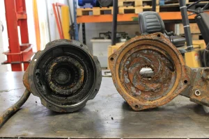
Figure 1: Particulate erosion causes severe material loss in industrial piping, making accurate CFD predictions vital for preventing catastrophic failures

Engineers must understand exactly where the material loss will happen and how fast it will occur. If erosion is not controlled, it will rapidly reduce the expected lifetime of expensive equipment and lead to catastrophic leaks. To solve this, engineers now rely heavily on advanced software like ANSYS Fluent to perform a complete CFD erosion simulation. Here is a quick guide comparing how engineers handle erosion problems:

Approach	Methodology	Limitation / Advantage
Physical Testing	Building prototype pipes and measuring wear over time.	Extremely expensive, very time-consuming, and involves too much trial and error.
API RP 14E Standard	Using simple empirical equations to set a “safe” maximum flow velocity.	Very limited. It cannot predict the exact location of the damage in complex geometries.
ANSYS Fluent CFD	Using computational models to track millions of particles and calculate surface wear.	Highly advantageous. It accurately predicts the exact location, shape, and severity of the erosion scar before any part is ever built!

Erosion Mechanisms: Particulate, Droplet, Cavitation & Corrosion

Industrial pipelines and hydrocarbon wells never transport pure fluids. They carry a highly chaotic multiphase mixture of oil, natural gas, water, waxes, and solid sand particles. When these complex mixtures travel at high speeds, they destroy piping infrastructure through four primary mechanisms.

To set up an accurate CFD erosion simulation, you must first identify which of these four mechanisms is destroying your geometry:

• Particulate Erosion: Solid particles like sand and proppant aggressively strike the pipe walls and carve away the metal. Particulate erosion is universally recognized as the absolute most common and destructive source of failure in oil and gas systems.
• Liquid Droplet Erosion: In wet gas systems, high-speed liquid droplets impact the walls like tiny bullets. However, this only causes severe damage at extreme velocities. The Salama-Venkatesh limit defines that significant droplet damage only occurs if the velocity exceeds .
• Cavitation Erosion: When the local fluid pressure drops below the vapor pressure inside a valve, vapor bubbles form. When these bubbles violently collapse near a wall, they generate massive micro-shock waves that instantly pit the metal.
• Erosion-Corrosion: This is a dangerous combination. Chemical corrosion weakens the surface metal, and the physical fluid flow immediately washes the weakened material away.

You must check the Cavitation Number (K) in your flow field. If K drops below 1.5, severe cavitation erosion is highly likely to occur alongside standard particle erosion. Because sand and proppant cause the vast majority of industrial pipeline failures, ANSYS Fluent is specifically designed to mathematically track these solid particles.

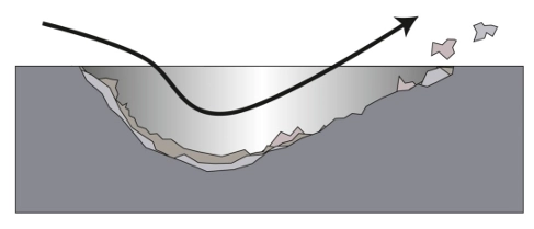
Figure 2: The process of removing layers of solid body over time by chaotic flow near the surface

Key Factors Affecting Particle Erosion

Particle erosion is not a random process. The exact amount of material removed from a pipe wall depends heavily on the fluid conditions, the physical shape of the particles, and the speed of the flow. To properly set up a CFD erosion simulation, engineers must first understand how these physical factors change the particle trajectories inside the domain.

The most critical factor in any erosion prediction is the particle impact velocity. Erosion rate is mathematically proportional to the particle velocity raised to an exponent (typically to for steel piping).

Because of this exponential relationship, even a tiny increase in the fluid flow speed will cause a massive increase in the wall damage! Here is a quick-guide table explaining how different physical properties directly control the erosion rate:

Physical Factor	How It Affects Erosion Behavior
Fluid Density & Viscosity	Dense, highly viscous fluids (like heavy oils) gently carry particles around corners, reducing impacts. Low-viscosity fluids (like natural gas) cannot turn the particles, causing them to travel in straight lines and aggressively crash into pipe walls.
Particle Size	Tiny particles (around 10 microns) safely follow the fluid streamlines. Very huge particles (around 1 mm) move too slowly or settle at the bottom. Medium-sized sand particles cause the most severe erosion damage because they carry high momentum and frequently hit the walls.
Particle Shape & Hardness	Hard sand particles remove significantly more metal than soft particles. Additionally, sharp, angular particles act like cutting tools, causing far more localized damage than smooth, rounded particles.
Flow Regime (Slugging)	Unsteady multi-phase flows often create slugs of liquid. These slugs generate periodic bursts of extremely high velocity, which drastically multiplies the erosion rate.

Gas systems are inherently much more dangerous for erosion than liquid systems. Because gas has very low density and operates at very high velocities, it provides almost zero cushioning effect to slow down the sand particles before they strike the metal surface.

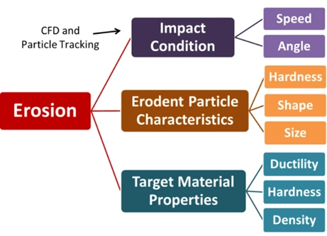
Figure 3: Erosion severity depends entirely on the fluid viscosity, particle shape, and impact velocity. Gas systems are far more prone to erosion due to the lack of a liquid cushion.

General Erosion Rate Expression & Variables

Before selecting any specific erosion model in ANSYS Fluent, you must understand the fundamental mathematics behind erosion calculation. ANSYS Fluent computes the erosion damage at wall boundaries using a master equation. Whenever a tracked particle hits a wall face, the software calculates the material loss using the General Erosion Rate Expression (Equation 15.8-1 in the Fluent Theory Guide):

Here is the simple breakdown of what every variable in this equation means:

Variable	Physical Meaning	How It Is Defined
	Erosion Rate	The total mass of material removed from the wall per unit area, per unit time.
	Particle Mass Flow Rate	The amount of sand or solid mass hitting the wall calculated by the DPM tracker).
	Diameter Function	A function that relates the particle size to the severity of the damage.
	Impact Angle Function	Defines how the impact angle changes the erosion. (e.g., direct 90° hit vs. a 20° grazing hit).
	Velocity Exponent	The particle impact velocity raised to a power. For most steel pipes,  is between 2 and 3.
	Wall Face Area	The physical area of the mesh cell face where the particle impacts.

It is critical to remember that the default units for Erosion Rate in ANSYS Fluent are . This represents mass flux, not physical depth! To understand the real-world lifespan of a pipe, engineers need the erosion rate in a unit of length over time, such as mm/year. To convert the default mass flux into mm/year, you must divide the calculated erosion rate by the physical density of the wall material using a Custom Field Function in Fluent’s post-processing tools.

 

Particle-Wall Interaction & Restitution Coefficients

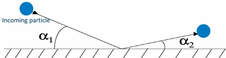
When a solid sand particle crashes into a steel pipe wall, it does not bounce off perfectly. The collision creates a tiny dent in the metal, which consumes a portion of the particle’s kinetic energy. Because the particle loses energy, its reflected velocity is always lower than its incoming velocity.

In ANSYS Fluent, this energy loss is mathematically calculated using Restitution Coefficients. You must define these coefficients to accurately predict where the particle will bounce next. For erosion simulations, the wall boundary condition in the DPM tab must always be set to Reflect. Once set to Reflect, you must define two separate coefficients:

Restitution Coefficient	Physical Meaning	Typical Behavior
Normal (Rn)	Controls how much speed the particle keeps in the perpendicular direction (bouncing straight off).	The lowest bounce energy usually happens at around a 40-degree impact angle.
Tangential (Rt)	Controls how much speed the particle keeps parallel to the wall (sliding along the surface).	The sliding energy gets lower as the impact angle gets steeper.

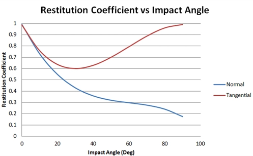
Figure 4: At impact, particles lose energy and bounce off at lower velocities. You must define Normal and Tangential Restitution Coefficients as polynomial functions of the impact angle.

Warning: The default setting for restitution coefficients in ANSYS Fluent is exactly 1.0 (a perfectly elastic collision). If you do not change this, your particles will bounce forever without losing energy, completely destroying the accuracy of your erosion prediction!

Fluent gives you several options for defining these coefficients:

• Constant (Not recommended for accurate erosion)
• Polynomial (Highly recommended. You input a mathematical equation based on the impact angle.)
• Piecewise-linear
• Piecewise-polynomial

In industrial simulations, engineers almost always select the Polynomial option. They input specific mathematical constants derived from experimental data for their exact pipe material (such as carbon steel or aluminum).

Figure 5: Discrete Phase Boundary condition panel in ANSYS Fluent

Impact Angle Function & Material Hardness

When a solid particle crashes into a wall, the severity of the damage is completely dependent on the angle of attack. A grazing hit at 15 degrees causes a very different type of wear than a direct, head-on crash at 90 degrees. In ANSYS Fluent, this physical behavior is mathematically defined by the Impact Angle Function, denoted as .

The shape of this mathematical function is entirely dictated by the physical hardness and metallurgical properties of your pipe wall. Wall materials are generally divided into two main categories:

• Ductile Materials (e.g., Carbon Steel, Aluminum): These softer metals suffer the most damage from shallow, grazing impacts. The maximum erosion rate for a ductile material always occurs at an impact angle between 20° and 30°. At these shallow angles, the sand particles act like a cutting tool, slicing thin layers of metal off the surface.
• Brittle Materials (e.g., Glass, Ceramics, Cast Iron): These extremely hard materials resist cutting but shatter under direct force. Therefore, the maximum erosion rate for a brittle material occurs at a direct, normal impact angle of 90°. The particles create deep micro-cracks that cause chunks of the material to simply fall out.

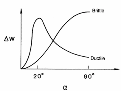
Figure 6: Ductile materials suffer maximum erosion at shallow angles (20°-30°), while brittle materials fail under direct 90° impacts. You must define this curve accurately using a piecewise-linear function.

You must input the correct angle function for your specific wall material. If you use a ductile angle function for a brittle ceramic wall, your entire CFD erosion prediction will fail!

It is also important to note that particle impact angles are heavily influenced by the concentration of particles in the fluid. In highly concentrated slurry flows, particles constantly collide with each other, forcing them to move parallel to the wall at very shallow angles. To accurately predict impact angles in these complex dense regimes, engineers must switch from standard particle tracking to advanced multiphase frameworks, such as the Eulerian Granular Model or a fully coupled DDPM-DEM simulation.

Figure 7: Free blogs focusing on DDPM & Grannular model approach in ANSYS Fluent

Overview of the Primary Erosion Models in ANSYS Fluent

ANSYS Fluent has a special Erosion Module inside the Discrete Phase Model (DPM) settings. Because every pipe material and fluid is different, you cannot use just one math formula for everything. So, the software gives you different models to choose from. You just need to select the one that matches your real-world problem.

Also, if you want to see how these models work in real examples, you can check out these different erosion projects:

• CFD Analysis of Particle Transport in Open Channel Flow (DPM Erosion Simulation in Ansys Fluent)
• Erosion in Air-Cooled Condenser (ACC) CFD Simulation (Ansys Fluent Training)
• Erosion in Centrifugal Fan CFD Simulation (Ansys Fluent Training)
• Erosion Inside Cyclone Separator CFD Simulation (Ansys Fluent Training)

Figure 8: Several CFD erosion projects performed by CFDLAND engineers

Here are the five main erosion models you will use in the software:

• The Generic Model: This is the basic option in Fluent. Because it is flexible, you can type your own math rules to tell the software how the particle size, speed, and hit angle change the damage.
• The Finnie Model: Engineers use this a lot for soft metals like carbon steel. To use it, you just need to enter the particle speed and the exact angle that causes the most wear.
• The McLaury Model: This model is made specially for water mixed with sand. So, it is great for predicting wear inside liquid pipes and valves.
• The Oka Model: This is a very detailed model. It uses the physical hardness of your pipe wall. To make it work, you need to type in exact test data and reference speeds from a real lab.
• The DNV Model: This model is very easy to set up. You just enter a number for the speed. After that, you just check a box to tell the software if your wall is soft (ductile) or hard (brittle).

Remember, default numbers in these models are often based on specific sand hitting carbon steel. Because of this, you should always change the numbers to match your own material.

Figure 9: ANSYS Fluent has specific input menus for the Generic, Finnie, McLaury, Oka, and DNV erosion models inside the DPM wall settings.

 

Setup for Finnie, McLaury & Oka Models

When you open the DPM wall settings in ANSYS Fluent, you must enter exact numbers for your chosen erosion model. Because every model uses a different math equation, you cannot skip any parameters. Here is the setup guide and the governing equation for the three most common models: Finnie, McLaury, and Oka.

The Finnie Model

Engineers use the Finnie model mostly for ductile metals like steel. It calculates the damage based on the kinetic energy of the particles.

• ER: Erosion Rate
• k: Empirical Constant
• V: Particle Velocity (Speed)
• n: Velocity Exponent
• f(alpha): Impact Angle Function

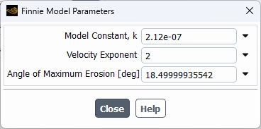
Parameters you must set in Fluent: To make this model work, you must open the Finnie Model Parameters window and enter these exact values:

• Model Constant (k): A base number from your material tests.
• Velocity Exponent (n): The default is 2. But, for metals, this number is usually between 2.3 and 2.5.
• Angle of Maximum Erosion: The exact angle where the most damage happens (usually between 20 and 30 degrees for soft metals).

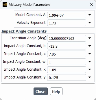
The McLaury Model

This model is perfect for water and sand mixtures. So, it is heavily used for liquid pipes and choke valves. It uses a very special angle function.

• ER: Erosion Rate
• A: Model Constant
• V: Particle Velocity
• n: Velocity Exponent
• f(alpha): Impact Angle Function (calculated using specific angle constants)

Parameters you must set in Fluent: Because this model is complex, you must enter many details in the McLaury Model Parameters window:

• Model Constant (A): A base multiplier.
• Velocity Exponent (n): Power of the particle speed.
• Transition Angle: The angle where the math function changes its shape.
• Impact Angle Constants: You must enter six different math constants: b, c, w, x, y, and z. These numbers shape the exact curve of the damage.

The Oka Model

The Oka model is very exact because it uses the real physical hardness of your pipe. It compares your real system to a basic reference test.

• ER: Erosion Rate
• E90: Reference Erosion Rate at a 90-degree angle
• V / Vref: Real speed divided by a reference speed
• D / Dref: Real particle size divided by a reference size
• k2 & ka: Velocity and Diameter Exponents
• f(alpha): Impact Angle Function

Parameters you must set in Fluent: First, you must have data from a real lab test. Then, you open the Oka Model Parameters window and enter:

• Reference Erosion Rate (E90): The damage seen in the lab.
• Wall Material Hardness: The exact hardness of your pipe (in Vickers Hardness).
• Model Constants (n1, n2): Numbers that adjust the angle function.
• Velocity Exponent (k2): Power for the speed ratio.
• Diameter Exponent (ka): Power for the size ratio.
• Reference Diameter (Dref): The sand size used in the lab test.
• Reference Velocity (Vref): The sand speed used in the lab test.

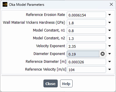
Figure 10: You must fill in every parameter in the DPM wall settings. The Finnie, McLaury, and Oka models each require specific constants and exponents.

Setup for DNV and Generic Models

In the last section, we learned about three models. Now, we will look at the DNV model, the Generic model, and a special model for dense flows. Because you need to know how they work, we will also show the basic math equation for each one.

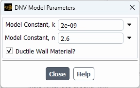
The DNV Model Setup

First, the DNV model is very popular in the oil and gas industry. It is very easy to use. The basic equation is:

Erosion Rate = K × Vⁿ × f(α)

(Where K is a constant, V is the particle speed, n is the velocity exponent, and f(α) is the impact angle function).

To set up this model, you only need to give the software three simple parameters:

• Model Constant (K): This is the base math number for the equation.
• Velocity Exponent (n): This number shows how much the speed increases the wear.
• Ductile Wall Material?: This is just a simple checkbox. You must check this box if your pipe is a soft metal (like steel). If your pipe is hard glass or ceramic, you leave the box empty.

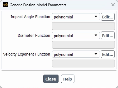
The Generic Model Setup

Next, the Generic model gives you total freedom. Because it is an open model, it does not use fixed numbers. The basic equation is:

Erosion Rate = Mass Flux × C(d) × f(α) × Vⁿ

(Where Mass Flux is the sand volume, C(d) is the diameter function, f(α) is the angle function, and Vⁿ is the velocity function).

To set this up, you must create your own math curves for these three parameters:

• Impact Angle Function: You must define how the hit angle changes the damage.
• Diameter Function: You must define how the sand size changes the damage.
• Velocity Exponent Function: You must define how the speed changes the damage. (Note: You can enter these as constant numbers, or use a piecewise-linear table to draw a custom curve).

Shear Stress (Abrasive Erosion) Setup

Finally, we have the Shear Stress model. This is used for very dense sand slurries. It calculates sliding wear instead of direct hits. The basic equation is:

Erosion Rate = A × τ × Vⁿ × (α_s / α_limit)

(Where A is a constant, τ is the wall shear stress, V is the sliding speed, and α_s is the sand volume).

Because it works with dense flows, you must type in these exact parameters:

• Velocity Exponent: The number that controls the sliding speed effect.
• Empirical Model Constant (A): The main math constant for the material.
• Solid Phase Packing Limit: The maximum amount of sand that can fit in one space (usually around 0.63).
• Granular Phase Shielding: This is a checkbox. You check this to tell the software that thick sand layers will protect the wall from more damage.

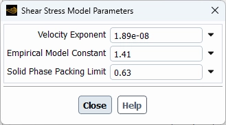
Figure 11: You must type the correct constants and math functions into the DNV, Generic, and Shear Stress setup boxes to get accurate erosion predictions.

Dense Systems: Abrasive Erosion & Wall Shear Stress

Most normal erosion models only calculate damage when a particle directly hits the wall. But, in heavy flows with a lot of sand, the particles do not just hit the wall and bounce off. Instead, they pack together and slide parallel to the pipe surface.

Because of this sliding motion, the particles scrape the metal like sandpaper. Engineers call this Abrasive Erosion. To calculate this special type of damage, ANSYS Fluent uses the Wall Shear Stress model. This model measures the actual friction force of the solid sand rubbing against the wall.

• ER: Abrasive Erosion Rate
• A: Empirical Model Constant
• Taw(ws): Solid Phase Wall Shear Stress (The friction force of the sand)
• Vs: Solid Phase Velocity (The sliding speed of the sand bed)
• n: Velocity Exponent

Also, when the sand is very thick, the particles crash into each other before they can reach the wall. Because of this, the wall is actually protected from direct hits. Engineers call this the Shielding Effect. ANSYS Fluent uses a second math rule to lower the normal impact damage based on how much sand is present:

• ER: The new, lower impact damage
• ER: The original damage calculated by models like Finnie or Oka
• Taw(ws): Volume Fraction of Solid Phase (How much sand is in the fluid)
• Vs: Solid Phase Packing Limit (The maximum sand concentration allowed)

So, your total damage in a dense system is the sum of both the sliding damage and the shielded impact damage

To use this advanced model, you must open the Shear Stress Model Parameters window in the DPM wall settings and enter these exact values:

• Velocity Exponent (n): The power of the sliding speed.
• Empirical Model Constant (A): A base multiplier for the friction damage.
• Solid Phase Packing Limit (Alpha(sp)): The maximum physical volume fraction of your sand bed (usually around 0.60 to 0.64 for spheres).
• Granular Phase Shielding: You must click and check this small box to turn on the protection effect for thick flows.

Single Phase vs Multiphase Erosion

When engineers run a simulation, they must choose between a single-phase flow and a multiphase flow. Because these two flows behave very differently, the damage results will also be very different.

First, single-phase erosion means you only have one fluid (like pure gas) carrying the sand. Because gas is very light and has low viscosity, the sand particles travel in straight lines. They do not slow down easily. So, they hit the pipe walls at very high speeds. As a result, single-phase simulations usually predict very high, conservative damage.

Next, multiphase erosion means you have a mix of gas, liquid, and sand (very common in oil and gas). Multiphase flows are very complex because the flow changes shape (like slug flow or annular flow). This creates two natural protections for your pipe:

• Liquid Cushion (Damping Effect): The liquid is heavy and thick. It creates a protective film on the pipe wall. So, the sand slows down before it hits the metal.
• Particle Shielding: In dense flows, many sand particles group together. Because the sand is so thick, the top layers of sand protect the wall from the other moving particles.

In conclusion, single-phase models are easier to set up, but they often show too much wear. Because real systems have liquid cushions and sand shielding, you must use multiphase simulations to get the true, lower erosion rates.

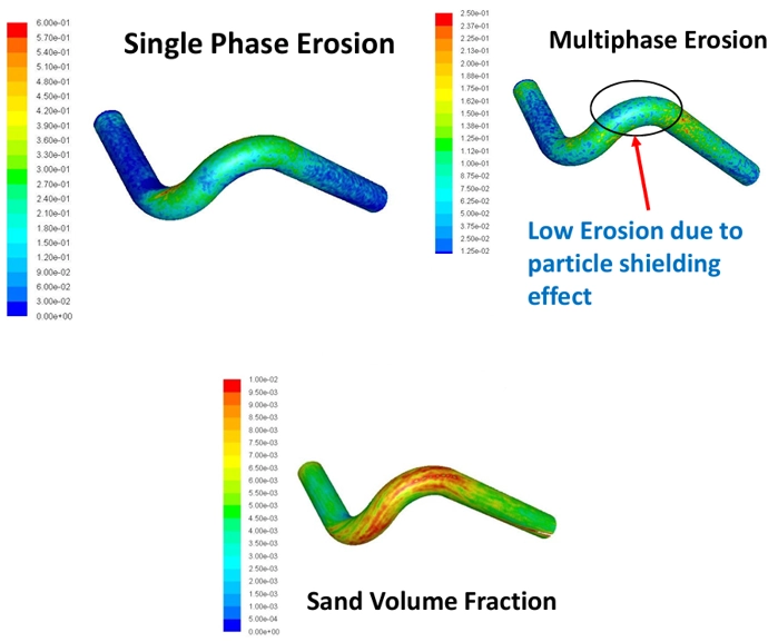
Figure 12: Single-phase simulations predict high wear, but multiphase simulations show less damage because the liquid layer acts as a protective cushion.

Erosion-Dynamic Mesh (MDM) Coupling Prerequisites

Normally, erosion models only calculate a damage number. But in real life, erosion removes actual metal and changes the shape of the pipe. To see this physical hole grow over time, ANSYS Fluent connects the erosion solver to the Moving/Dynamic Mesh (MDM) tool. First, this physical wear is a very slow process. So, Fluent uses a “quasi-steady” method. This means it solves the steady flow, calculates the damage, and then moves the mesh nodes to show the lost metal.

Governing Equation for Mesh Deformation:

• Delta(n): Mesh Deformation (how much distance the wall moves)
• ER: Erosion Rate Density (the damage rate)
• rho(wall): Wall Material Density (the physical weight of the pipe metal)
• Delta(t): Mesh Motion Time Step Size

Before you can run an MDM coupling simulation, you must follow these exact rules:

• Steady State Flow: You must use a steady-state flow solver.
• Absolute Tracking: You cannot use “Relative particle tracking.” You must track all sand particles in the absolute frame.
• Wall Material Density: You must type in the correct density for your pipe. (The software default is 2719 kg/m³ for aluminum. If you use steel, you must change this to around 7850 kg/m³).
• Smoothing and Remeshing: Because the wall moves, the mesh cells will stretch. So, you must turn on the Smoothing and Remeshing methods to keep the mesh quality high.
• Initial Flow Field: You must run a normal flow simulation and get a converged result before you turn on the moving mesh.

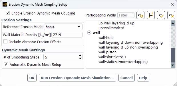
Figure 13: To physically deform the wall, you must use the Erosion Dynamic Mesh menu and enter the correct Wall Material Density.

Executing the Simulation & Post-Processing Results

Now you are ready to run the moving mesh simulation and view your final results. Because this is a special coupled solver, you cannot use the normal run button! First, you must open the special “Run Erosion-Dynamic Mesh Simulation” window. Here, you set your time controls.

• It is best to choose a variable-time-step. This lets the software control the speed based on the “Maximum Node Movement.” A good starting number is 10% to 30% of the cell length.
• Next, you type in your Total Time of Erosion (for example, the seconds in a full year).
• Also, you can use the “Autosave Graphics” option. This tells Fluent to automatically save pictures of the mesh at every step so you can make a nice animation later.

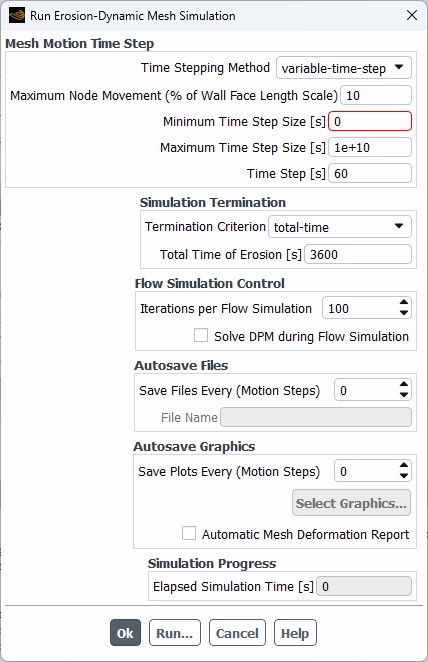
Figure 14: Run erosion-dynamic mesh simulation panel

After the simulation finishes, you want to see exactly how much metal was removed. Normal erosion models only show you a rate (like kg/m²s). But, because you used MDM, you can see the true physical shape change.

To see this new shape, you go to the post-processing contour menu. Instead of looking at the standard erosion variables, you must look under the Mesh category and select Accumulated Deformation. This will show you exactly how many millimeters of material the sand removed from your pipe wall.

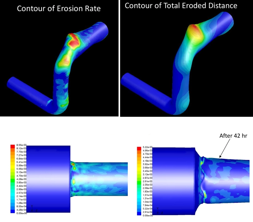
Figure 15: By looking at the Accumulated Deformation, you can physically see the new shape and calculate the exact material thickness lost.

As an other case in a point, please check Erosion-MDM simulation performed by CFDLAND, focused on oil pipes. To calculate the realistic, long-term metal damage, we applied the powerful Erosion-MDM coupling. This means we combined the McLaury erosion equations with the Dynamic Mesh Module (MDM).

Conclusion

To sum up, predicting erosion in ANSYS Fluent is very important to protect pipes and valves from sand damage. First, you must choose the correct setup, like the Finnie, McLaury, or Oka model. Next, for heavy sand flows, you must use multiphase simulations to get the most realistic results. Finally, you can connect your model to the Dynamic Mesh (MDM) to physically see the metal wear away over time!

If you need help with your CFD simulations, you can use our Order Project service. Our experts are masters of erosion! We provide effective strategies and solutions to tackle your toughest erosion challenges and ensure your project is a complete success.