

Welcome to our guide on Radiation Heat Transfer in ANSYS Fluent. While conduction and convection are familiar heat transfer modes, radiation is a unique and powerful mechanism. It is the transfer of energy through electromagnetic waves and, unlike the other two modes, it does not require a medium to travel through. This is why we can feel the heat from the sun, even through the vacuum of space.
What is Radiation and When is it Crucial in CFD?
In the world of CFD simulation, we often ask: when must we include Radiation CFD effects? The answer is simple: at high temperatures. The energy radiated from a surface is proportional to its temperature raised to the fourth power (T⁴), as described by the Stefan-Boltzmann Law. This means that as temperatures increase in applications like combustion, furnaces, glass manufacturing, or solar load analysis, the contribution of Fluent Radiation quickly becomes dominant, far outweighing conduction and convection. Ignoring it can lead to completely wrong results.
ANSYS Fluent provides a comprehensive set of tools to model these complex phenomena. Whether the heat is traveling through a transparent medium (non-participating) or through a fluid that absorbs, emits, and scatters energy (a participating medium), there is a model to handle the simulation. To learn more about our projects and tutorials, you can explore our advanced radiation CFD simulation tutorials.

Figure 1: A showcase of advanced Radiation CFD simulation tutorials available from CFDLAND, demonstrating the diverse applications of the ANSYS Fluent radiation module.
The Physics of Radiation: Blackbody, Gray Body, and Emissivity
To correctly set up a Radiation CFD simulation, we must first understand the basic physics of how surfaces radiate energy. This involves a few key concepts that are fundamental to all thermal radiation calculations.
Black Body Radiation
A black body is an ideal, theoretical object. It is defined as a perfect radiator that absorbs 100% of all radiation that strikes it, reflecting and transmitting none. Because it is a perfect absorber, it is also a perfect emitter. The energy emitted by a black body is the theoretical maximum possible for a given temperature and is described by the Stefan-Boltzmann Law:

Here, q is the heat flux, σ (Sigma) is the Stefan-Boltzmann constant, and T is the absolute temperature. This T⁴ relationship is why ANSYS Radiation becomes so important at high temperatures.

Figure 2: An illustration of a blackbody, the ideal object that absorbs all incident energy and acts as a perfect emitter, a fundamental concept in thermal radiation heat transfer.
Gray Body Radiation
In the real world, no object is a perfect black body. Real objects are often modeled as gray bodies. A gray body emits less radiation than a black body at the same temperature. The main difference between a gray body and a black body is defined by a property called emissivity (ε). Emissivity is a crucial property in Radiation Heat Transfer. It is a value between 0 and 1 that describes the ratio of the energy radiated by a real surface to the energy that would be radiated by a black body at the same temperature.
- For a perfect black body, ε = 1.
- For a gray body, 0 < ε < 1.
- For a perfect reflector, ε = 0.
The net radiative heat transfer between a small gray body and its large surroundings can be expressed as:

Where ε is the surface emissivity, A is the surface area, and T are the temperatures of the wall and surroundings. For most Fluent Radiation simulations, defining the correct emissivity for your materials is one of the most important steps to getting an accurate result.
Governing Equation: Understanding the Radiative Transfer Equation (RTE)
At the heart of every Radiation CFD simulation in ANSYS Fluent is a complex governing equation. This is the Radiative Transfer Equation (RTE). While you don’t need to solve it by hand, understanding what it represents is crucial for choosing the right simulation settings.
In simple terms, the RTE is an energy balance equation for a single ray of radiation as it travels through a medium. It calculates how the intensity of that radiation changes along its path. The RTE accounts for all the physical phenomena that can increase or decrease the ray’s energy.
The main components considered in the RTE are:
- Emission: Energy that is added to the ray because the fluid or gas itself is hot and is emitting its own radiation.
- Absorption: Energy that is lost from the ray because it is absorbed by the surrounding fluid.
- Out-Scattering: Energy that is lost from the ray because particles in the fluid cause it to scatter in a different direction.
- In-Scattering: Energy that is gained by the ray because radiation from other directions is scattered into its path.
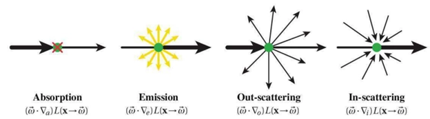
Figure 3: Emission, Absorption, Out-Scattering, and In-Scattering affecting the ray.
Solving the full Radiative Transfer Equation is very computationally expensive. This is why ANSYS Radiation provides different radiation models, such as the P1, DO (Discrete Ordinates), and S2S (Surface-to-Surface) models. Each of these models uses a different mathematical method to simplify and solve the RTE, making the radiation simulation practical for engineering problems.
Key Concepts for Fluent: Participating Media and Optical Thickness
Now that we understand the governing Radiative Transfer Equation (RTE), we need to define the properties of the environment the radiation is traveling through. Two of the most important concepts for any ANSYS Fluent Radiation simulation are how surfaces interact with radiation and whether the fluid medium itself plays a role.
Surface Interaction: Absorption, Reflection, and Transmission
When a ray of radiation (called incident radiation) strikes any surface, such as a wall, it can be divided into three parts:
- Absorption (α): A fraction of the radiation is absorbed by the surface, increasing its internal energy and temperature.
- Reflection (ρ): A fraction of the radiation bounces off the surface.
- Transmission (τ): A fraction of the radiation passes straight through the surface, only possible if the material is semi-transparent (like glass).
The sum of these three fractions must always equal one, representing 100% of the incoming energy. The equation is:
α + ρ + τ = 1
For most engineering problems in CFD simulation, we deal with solid, opaque surfaces. For an opaque surface, there is no transmission (τ = 0), which simplifies the relationship to: α + ρ = 1 This means any radiation that hits the surface is either absorbed or reflected.

Figure 4: How radiation heat transfer interacts with an opaque surface in a CFD simulation, where incident energy is divided between absorption (α) and reflection (ρ).

Figure 5: The interaction of radiation with a semi-transparent surface, like glass, in ANSYS Fluent, showing how energy is split into absorption (α), reflection (ρ), and transmission (τ).
Participating vs. Non-Participating Media
In Radiation CFD, the fluid itself can be one of two types:
- A non-participating medium is completely transparent to radiation. It does not absorb, emit, or scatter energy. Think of a vacuum or air at room temperature. In this case, radiation only travels from one surface to another without being affected by the fluid in between. The S2S (Surface-to-Surface) model in Fluent is designed for this scenario.
- A participating medium is a fluid that actively interacts with radiation. It can absorb, emit, and scatter radiation as it passes through. This is extremely important in applications like combustion, where hot gases like CO₂ and water vapor, along with soot and smoke, significantly affect the radiation heat transfer.
How to Measure Interaction: Optical Thickness
So, how do we know if a medium is participating or not? We use a dimensionless parameter called Optical Thickness. It tells us how opaque a fluid is to radiation over a certain distance.
- An optically thin medium (optical thickness << 1) is nearly transparent. Radiation can travel a long way through it without being absorbed.
- An optically thick medium (optical thickness >> 1) is nearly opaque. Radiation is absorbed very quickly over a short distance.
There are two main ways to understand and calculate optical thickness:
- Based on Intensity: Conceptually, optical thickness (τ) is the natural logarithm of the ratio of incident radiation (I₀) to the transmitted radiation (I). This shows how much the radiation intensity is reduced as it passes through the medium.

- Based on Material Properties: In practice for ANSYS Fluent setups, the optical thickness is calculated by multiplying the medium’s absorption coefficient (a) by the characteristic path length (L) of the domain.

This value is what you will use to decide which radiation model is best. For example, if the optical thickness is very large (a * L > 3), the Rosseland model is a good choice. If it is very small, the S2S model might be appropriate (if the medium is non-participating). Models like DO can handle a wide range of optical thicknesses.
An Introduction to the Radiation Models in ANSYS Fluent
ANSYS Fluent does not solve the full Radiative Transfer Equation (RTE) for every case because it would be too computationally expensive. Instead, it provides a suite of different radiation models, each with its own method of simplifying the RTE. Choosing the correct model is the most important decision in a Radiation CFD setup and depends on the physics of your problem, especially the optical thickness.
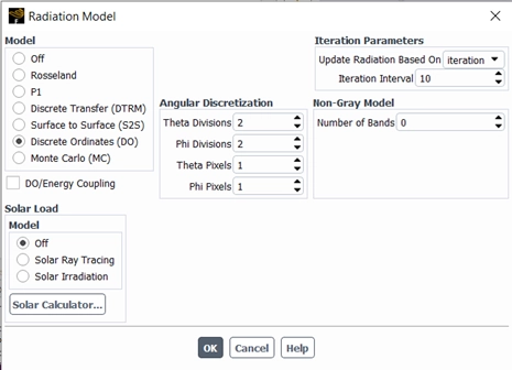
Figure 6: The selection panel for Radiation models within the ANSYS Fluent software, where users choose the appropriate method, such as the DO, P1, or S2S model, for their simulation.
Below is a summary table to help you understand the advantages and limitations of each primary ANSYS Radiation model.
| Radiation Model | Best For / Key Application | Key Advantages | Key Limitations |
| Discrete Ordinates (DO) | The most versatile model for the full range of optical thicknesses, from surface-to-surface to participating media like combustion. Ideal for semi-transparent walls. | • Spans all optical thicknesses. • Moderate computational cost. • Can solve radiation at semi-transparent walls. |
• Can be CPU-intensive with fine angular settings. • Assumes gray radiation (or non-gray band models). |
| P-1 Model | Combustion simulations and other applications with optically thick media and complex geometries. | • Low CPU demand. • Includes the effect of scattering. • Easy to apply to complex geometries. |
• Assumes diffuse surfaces. • Can lose accuracy in optically thin media. • Tends to over-predict flux from local heat sources. |
| Rosseland Model | Only for optically thick media (optical thickness > 3), such as radiation within solid glass. | • Very fast and requires less memory than the P-1 model. | • Cannot be used for optically thin or moderate media. • Only available with the pressure-based solver. |
| Surface-to-Surface (S2S) | Enclosure radiation with a non-participating medium, like spacecraft heat rejection or solar collector systems. | • Very fast time per iteration compared to DO and DTRM. | • Cannot be used with a participating medium. • Assumes diffuse & gray surfaces. • Memory needs increase rapidly with more surfaces. |
| Discrete Transfer (DTRM) | A simple model that can be applied to a wide range of optical thicknesses. | • Relatively simple to set up. • Accuracy can be improved by increasing the number of rays. |
• Does not include scattering. • Assumes all surfaces are diffuse. • CPU-intensive with many rays. |
In addition to these models, ANSYS Fluent also offers a Solar Load Model to specifically account for the effects of solar radiation. In our next blog, we will explore each of these models in detail, discussing their settings and providing practical examples to help you select the best one for your specific CFD simulation.
Conclusion
Radiation is a powerful and essential mode of heat transfer, especially in high-temperature applications where it often becomes the dominant factor. Setting up a successful Radiation CFD simulation in ANSYS Fluent requires a solid understanding of the fundamental physics, from emissivity and the Radiative Transfer Equation to key concepts like participating media and optical thickness.
As we have seen, ANSYS Fluent provides a range of specialized radiation models, from the simple Rosseland model to the versatile DO model. The most critical step in your simulation is selecting the correct model based on the physics of your problem. This choice will determine the accuracy and efficiency of your results. In our next blog, we will explore each of these models in greater detail, providing practical guidance on how to choose and implement them for your specific engineering challenges.