Axial fans are key components in many air-moving devices because they can quickly move large amounts of air along the fan’s rotational axis. These machines have a hub in the middle and blades that stick outward. As the blades rotate, they create a pressure gradient that moves air. Many industries use axial fans because they work very well in low-pressure situations. They are used in everything from home appliances and car cooling systems to workplace ventilation and HVAC systems. Because they are small, they can easily be installed in tight areas, which makes them perfect for uses that need straight-line airflow. In the present study, a 3D axial fan is investigated under guidance of reference paper entitled “ Reducing the aerodynamic noise of the axial flow fan with perforated surface “.

• Reference [1]: Yadegari, Mehdi, et al. “Reducing the aerodynamic noise of the axial flow fan with perforated surface.” Applied Acoustics215 (2023): 109720.

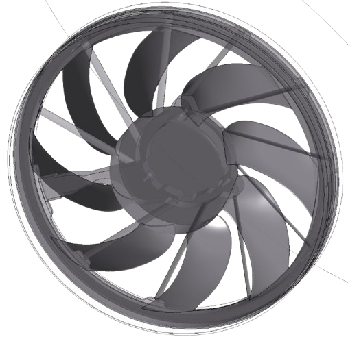
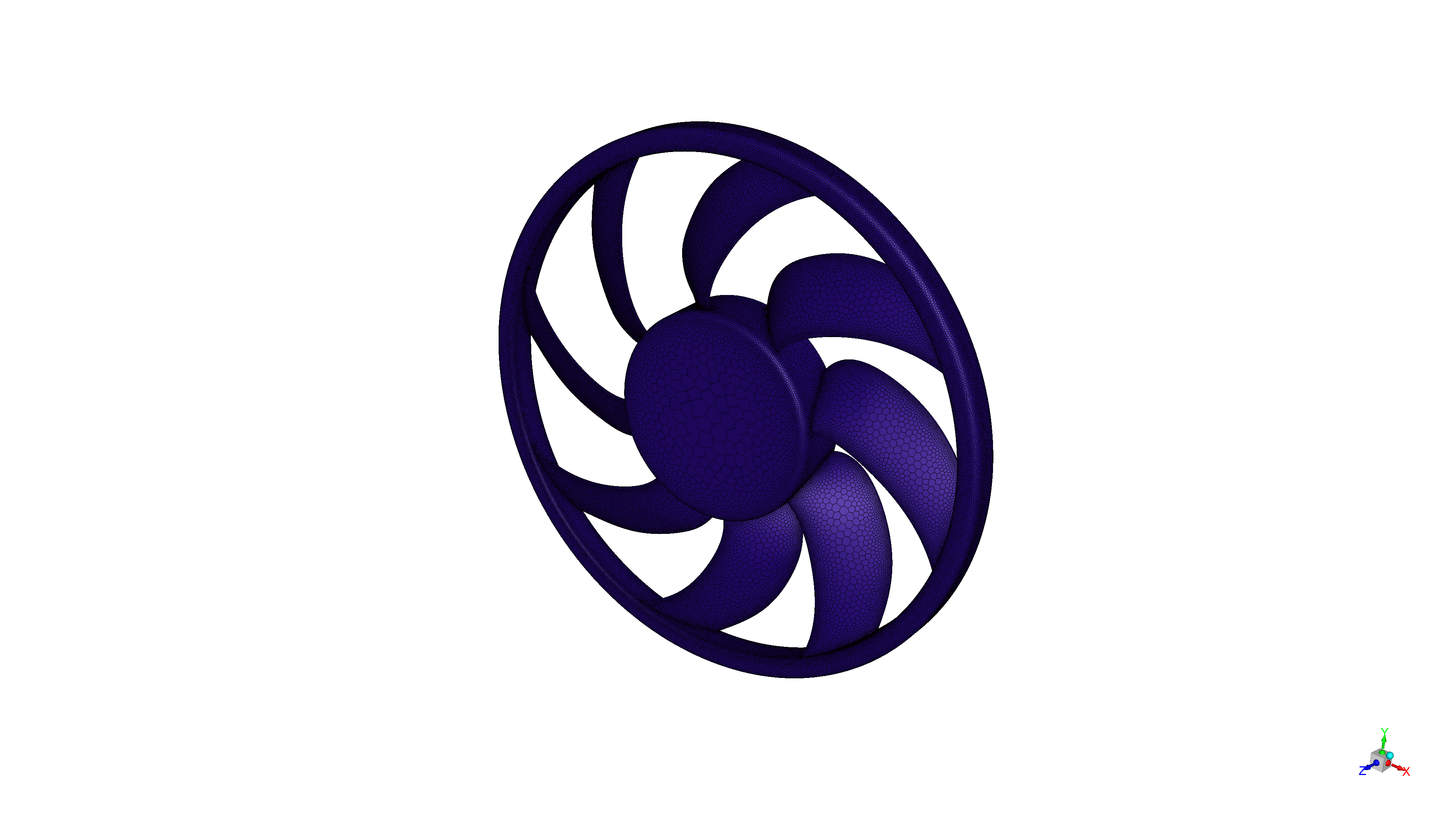
Figure 1: Schematic of 3D axial fan CFD Simulation

Simulation Process

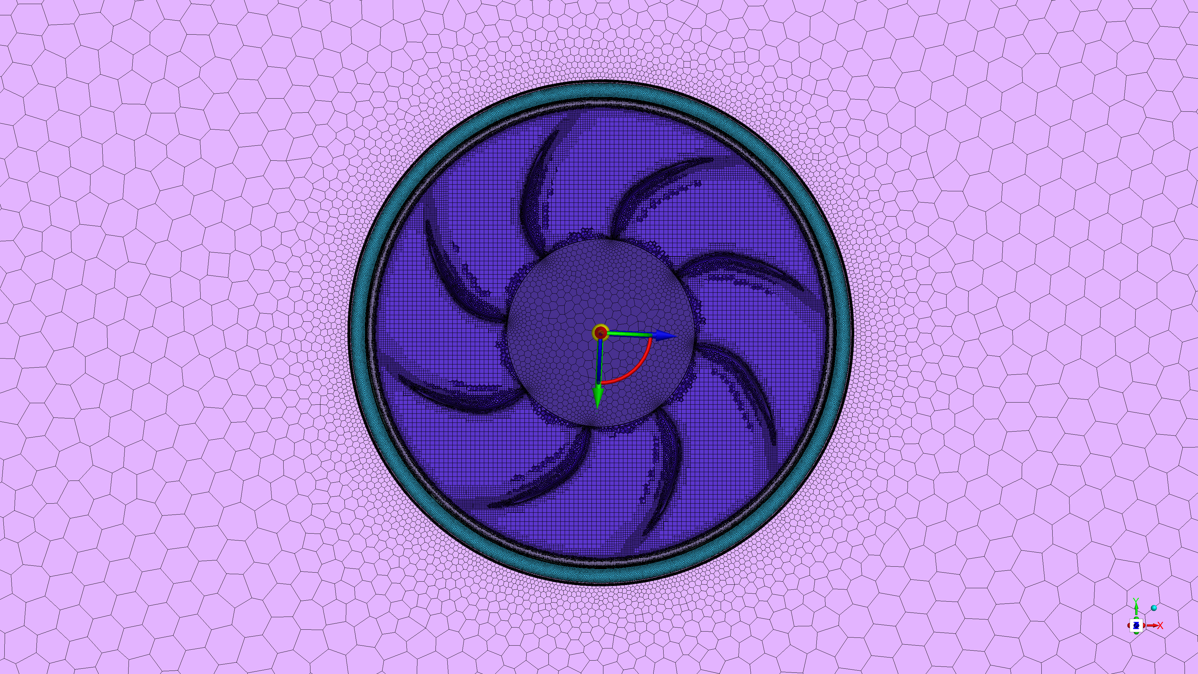
There are two separate domains in the simulation: a smaller circular region containing a fan rotor and a bigger domain around it representing the surroundings and the shroud. Next, the model is descritized into 4889858 polyhedral cells as shown in Fig. 2. The multiple reference frames (MRF) method is used to model rotating machines like turbines and pumps in steady aerodynamic simulations. The fan is rotating with 2818rpm angular velocity. The SST k-ω model is utilized to account for the turbulent nature of the flow according to the reference paper.

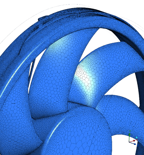
Figure 2: Polyhedra grid over 3D Axial Fan CFD Simulation

Post-processing

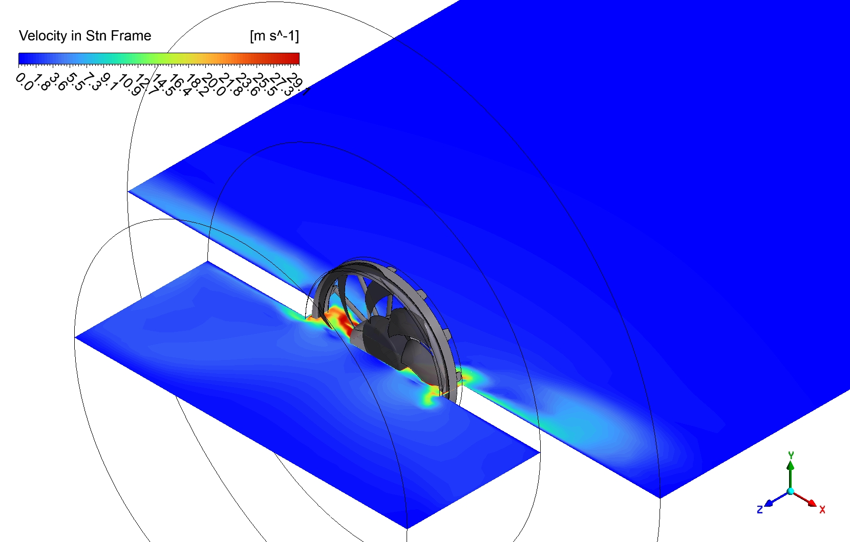
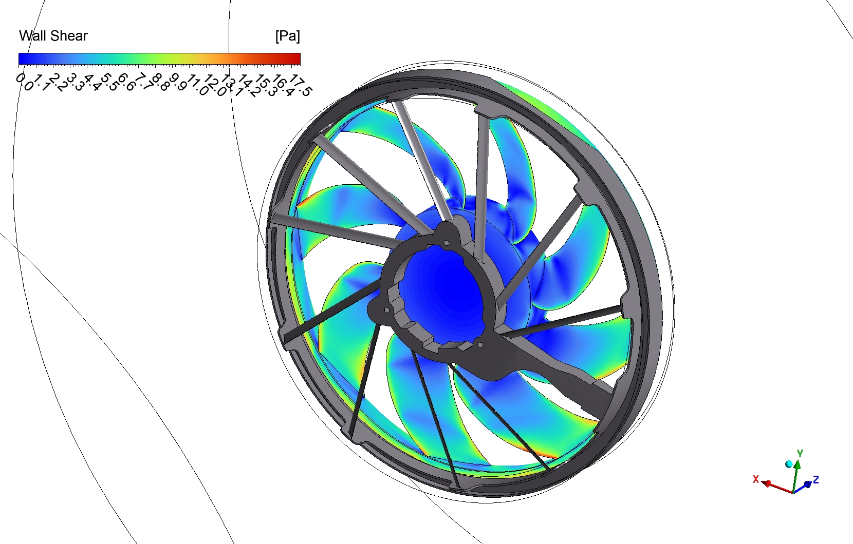
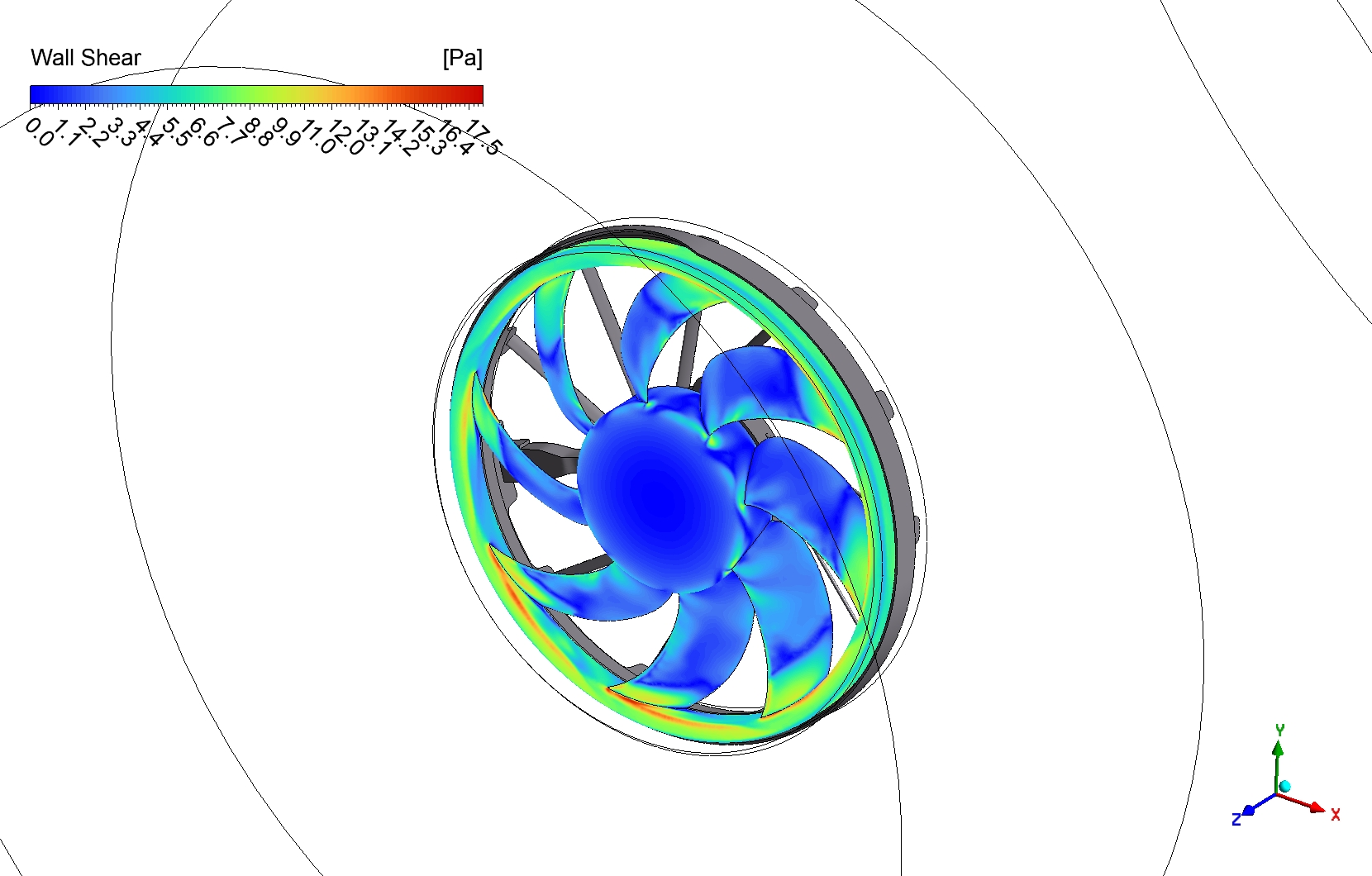
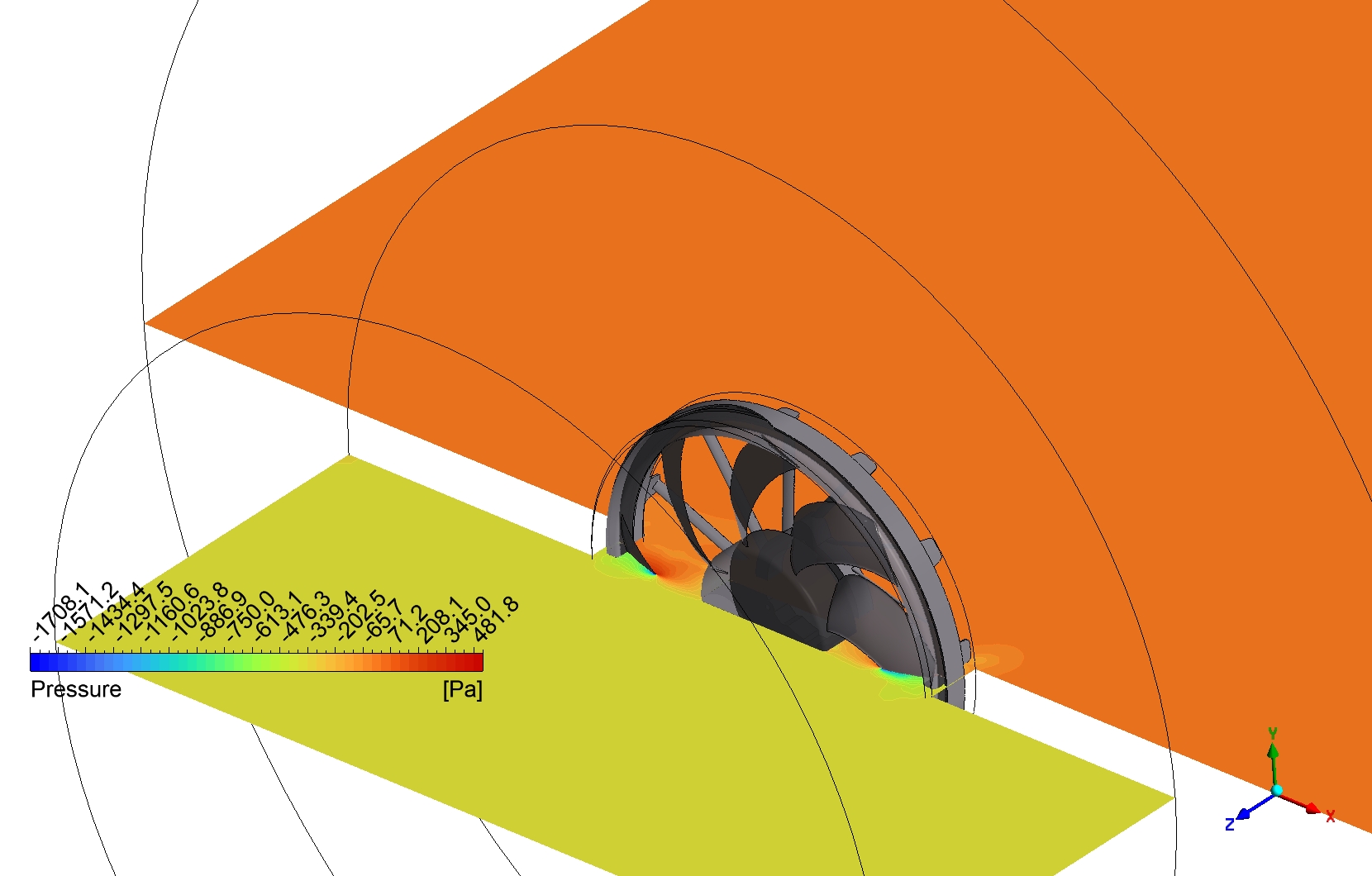
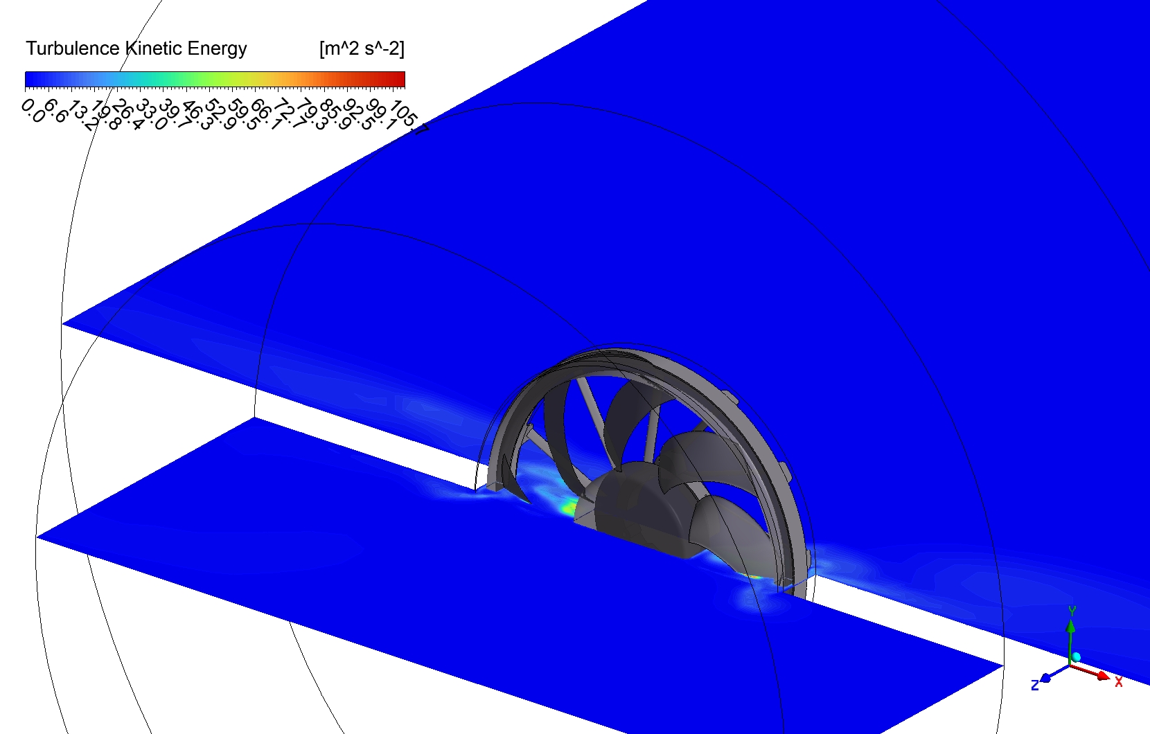
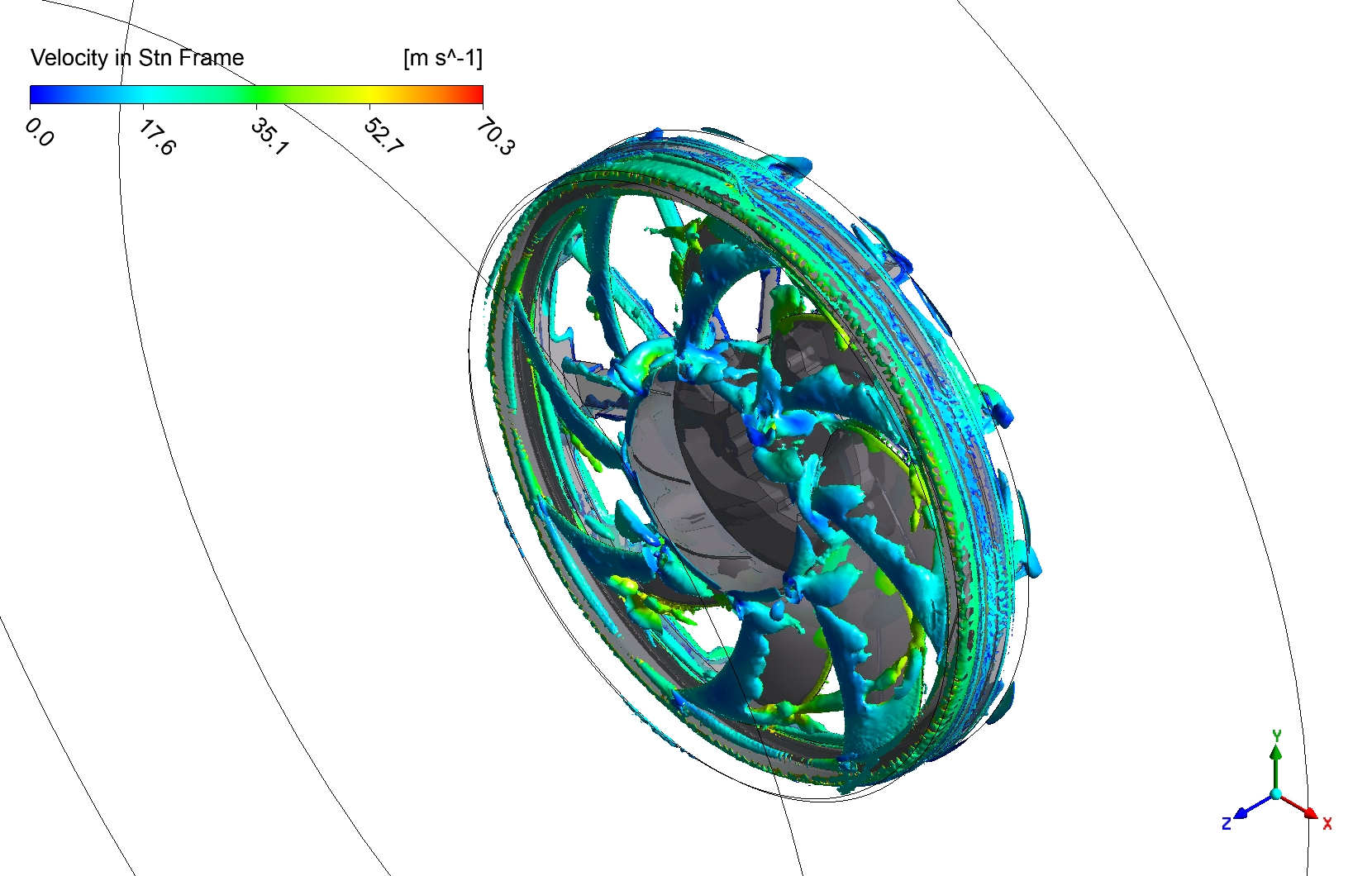
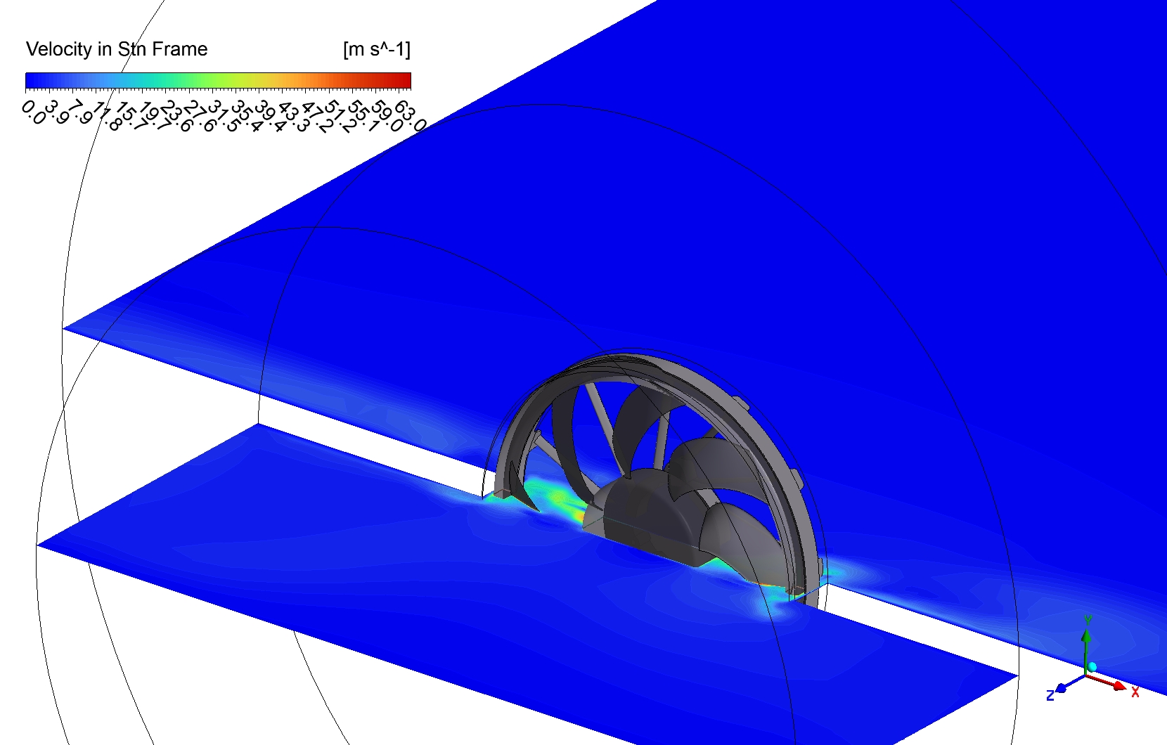
The 3D modeling of the axial fan running at 2818 rpm shows us a lot about how well it works. The range of speeds shown in the velocity contour, from 0 to 70.3 m/s, shows the complicated flow patterns inside and around the fan. The fastest speeds, shown by green to red areas, can be found near the fan’s blade tips and around its outside edge, reaching up to 70.3 m/s. The center hub area and areas between the blades, on the other hand, have slower speeds, which is shown by blue colors. This is how flow usually behaves in axial fans. The torque coefficient (cm) of 10.93 indicates that a lot of torque is being generated, which means that the fan can beat air resistance and keep turning at the same speed. High-pressure gradients and more vorticity are likely to be present in places where speeds change quickly, especially near the blade surfaces and tips. These areas, which can be seen as sharp changes between color bands, show possible places where the flow could split and vortices could form. The shear stress is likely to be strongest where there are steepest velocity gradients. This is usually along the blade surfaces and where the fast flow near the blade tips meets the slower air in the fan’s wake. In the middle of the fan, there were a lot of different-speed streams interacting with each other. This suggests that there is turbulent mixing and possible energy losses, which could affect how well the fan works overall.

Figure 3: Vorticity field around 3D axial fan CFD Simulation

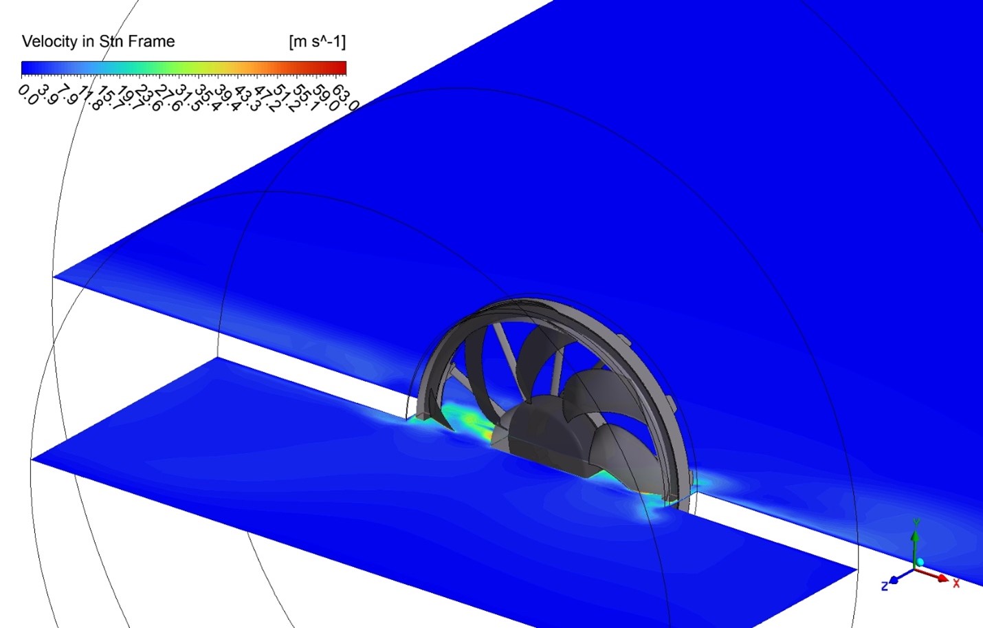
Figure 4: Velocity distribution around 3D axial fan CFD Simulation