In this CFD Analysis of Sinusoidal Motion of Wall tutorial, we explore how to simulate moving boundaries in engineering. In nature, many surfaces move to push fluids, such as a beating heart or the flapping wings of a bird. In mechanical engineering, vibrating pumps and micro-mixers use similar oscillating walls. To design these systems, we cannot assume the walls are stationary. We must use Sinusoidal Motion of Wall CFD methods. This approach simulates a wall that moves back and forth in a smooth, wave-like pattern, allowing us to calculate the resulting airflow or water flow.

The critical tool for this simulation is the Dynamic Mesh fluent capability. Standard CFD simulations use a fixed grid, but for this case, the mesh must stretch and compress as the wall moves. We also utilize a User Defined Function (UDF). This is a small script written in C language that tells ANSYS Fluent exactly how to move the wall over time. This Sinusoidal Motion of Wall fluent simulation is vital for manufacturers. It helps them predict flow patterns and forces that are impossible to see with the naked eye, ensuring that biological devices or cooling systems work correctly. For more details on moving grid setups, please explore our Dynamic Mesh tutorials.

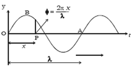
Figure 1: Schematic diagram of a Simple Harmonic Progressive Wave, illustrating the mathematical concept of the sinusoidal motion used for the wall boundary.

Simulation process: Dynamic Mesh Setup and UDF Implementation

For this CFD Analysis of Sinusoidal Motion of Wall, we began by creating a 2D channel geometry. The mesh generation is the most critical step for moving boundary problems. We generated an unstructured triangular mesh. We specifically refined the cells near the moving wall. Triangular cells are preferred here because they can handle the squeezing and stretching of the domain better than square cells without failing. To drive the motion, we wrote a specific UDF code. This code forces the wall to follow the equation with an amplitude () of 0.05 meters and a frequency of 1 Hz.

We configured the Dynamic Mesh fluent model to handle the grid deformation. We selected the Smoothing Method. This treats the edges of the mesh cells like springs; when the wall moves, the “springs” compress or expand to absorb the motion. Because the amplitude (0.05m) was relatively small compared to the domain size, we did not need to use “Remeshing.” This saves computational time. We set up a Transient Solver (unsteady) with very small time steps. This is necessary to accurately capture the changing velocity as the wall accelerates and decelerates through its cycle.

Post-processing: CFD Analysis of Sinusoidal Motion of Wall and Flow Evolution

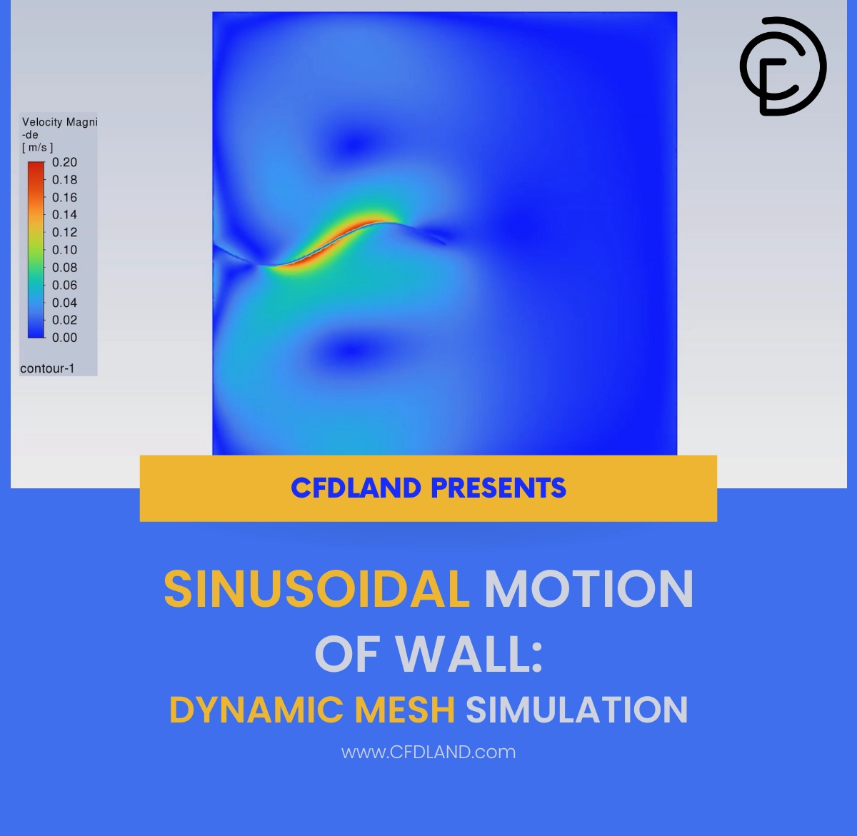
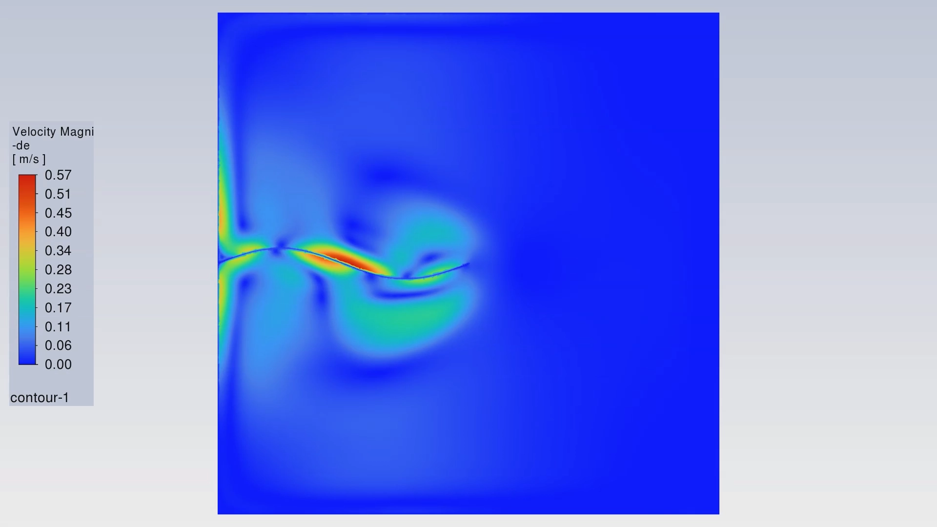
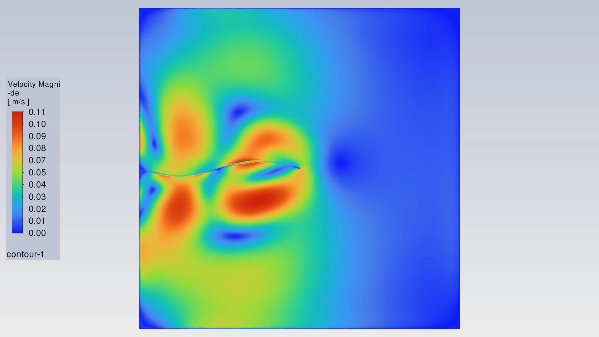
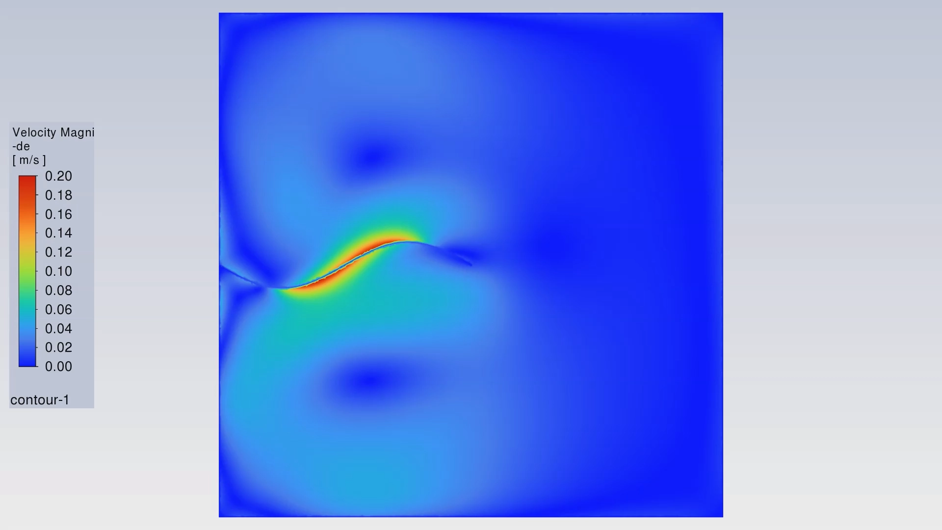
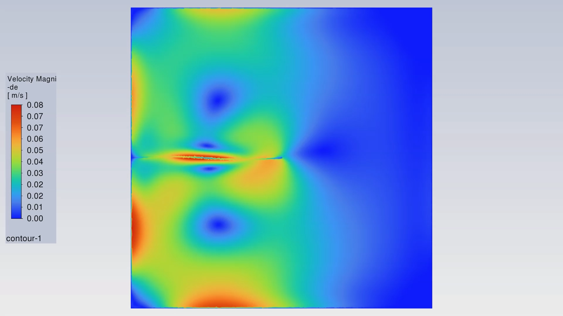
In this section, we perform a deep engineering analysis of the results. We interpret the contours to understand how the oscillating wall drives the fluid momentum. First, we analyze the Velocity Evolution in Figure 2. These four images show the history of the flow during one oscillation cycle. In the top-left image, the wall has just started moving. The velocity is very low, reaching only 0.08 m/s (Blue zone). As time progresses, the wall accelerates. By the final image (bottom-right), the Maximum Velocity reaches 0.57 m/s. Engineering Insight: This represents a velocity increase of over 700%. The contours show the high-velocity region (Red) growing from a thin strip near the wall into a large, complex wave pattern. This proves that the wall is effectively transferring kinetic energy to the fluid. It also demonstrates Fluid Inertia: the fluid does not stop instantly when the wall direction changes; instead, the momentum carries it forward, creating complex mixing layers.

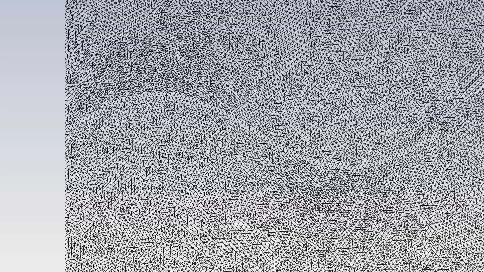
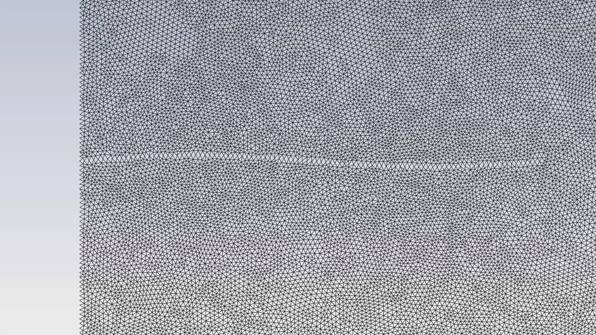
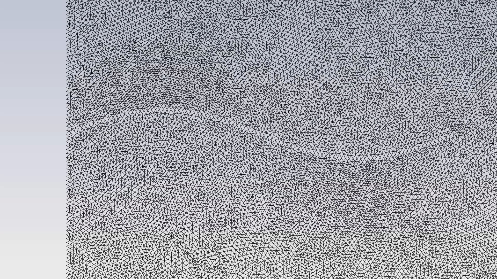
Next, we evaluate the Flow Mixing and Stability. The final contour shows a wavy, chaotic pattern where high-speed and low-speed zones are mixed. For a manufacturer, this is a Critical Benefit. If this device were a micro-mixer, this chaotic pattern would be excellent for mixing two chemicals together rapidly. Finally, we must verify the reliability of the simulation by checking Figure 3. This image shows the mesh before and after the movement. Although the triangles have stretched, they have not collapsed or inverted (No Negative Volumes). This confirms that our Dynamic Mesh ANSYS fluent strategy using the Smoothing method was robust and accurate for this amplitude.

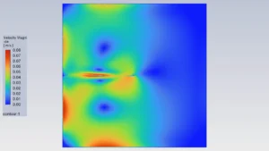
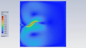
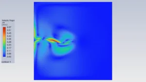
Figure 2: Velocity magnitude contours at four time instants during one complete sinusoidal oscillation showing the development of flow momentum.

Figure 3: Unstructured mesh with triangular elements for sinusoidal motion of wall CFD simulation in ANSYS Fluent; left shows initial mesh, right shows deformed mesh.

Key Takeaways & FAQ

• Q: Why is a UDF needed for this simulation?
  • A: Standard Fluent settings allow constant velocity, but a UDF is required to define a complex mathematical formula like a Sine Wave () for the wall motion.
• Q: Why use Triangular Mesh instead of Quad?
  • A: Triangular meshes are more flexible. In Dynamic Mesh simulations, triangles can stretch and skew more than quads without causing “Negative Volume” errors.
• Q: What is the main application of this analysis?
  • A: It is used for diaphragm pumps, flapping wing aerodynamics, and micro-fluidic mixers where walls are not stationary.