
What is Computational Fluid Dynamics?
Computational fluid dynamics (CFD) is an advanced branch of fluid mechanics that uses numerical methods and computer algorithms to solve and analyze problems involving fluid flows. In simple words, CFD helps engineers and scientists predict how liquids and gases will behave and interact with surfaces without actually testing them in real life! Furthermore, computational fluid dynamics simulation allows us to see what happens when fluids flow around objects or inside complex systems.
How CFD works is quite fascinating. First, engineers create a digital model of the object or system they want to study. Then, they divide this model into thousands or even millions of tiny cells (called a mesh). Next, powerful computers solve mathematical equations for each of these cells to calculate the movement, temperature, and pressure of the fluid. Finally, the results are displayed as colorful images or animations that show exactly how the fluid moves. The field of computational fluid dynamics has grown tremendously in recent decades. In fact, modern CFD programs can simulate incredibly complex situations that would be impossible to test physically. Additionally, computational fluid dynamics analysis helps designers improve their products by testing many different designs quickly and cheaply on the computer.
Historical Evolution of CFD | Computational Fluid Dynamics
The journey of computational fluid dynamics began in the early 20th century, but it wasn’t until the 1960s that significant progress was made. At that time, limited computing power meant that only very simple CFD simulations were possible. However, as computers became more powerful, so did the capabilities of CFD analysis.
In the 1970s, the aerospace industry started using basic computational fluid mechanics to help design aircraft. By the 1980s, automotive companies began adopting CFD modeling techniques too. Furthermore, the 1990s saw a boom in commercial CFD software that made these tools available to more engineers.
Today, computational fluid dynamics programs are used in virtually every industry from medicine to sports equipment design. Moreover, what once required supercomputers can now often be done on powerful desktop machines or through cloud computing services. In fact, the continuous improvement in computing power has revolutionized how we approach fluid flow simulation.

Figure 1: Dudley Brian Spalding – one of the founders of computational fluid dynamics (CFD)
Governing Equations and Mathematical Methods in CFD
Computational fluid dynamics (CFD) is built on fundamental equations that describe fluid motion. At its core, CFD simulation solves the Navier-Stokes equations, which represent mass, momentum, and energy conservation principles. These equations are incredibly complex, which is why powerful computers and specialized CFD programs are essential. Want to understand the theoretical foundation of CFD analysis in detail? Check out our comprehensive guide to The Essential Fluid Dynamics Equations where we break down each equation and explain their significance.
In practical computational fluid dynamics, these continuous equations are converted into discrete forms that computers can solve. This process, called discretization, divides the flow domain into thousands or millions of small cells. Various numerical methods like Finite Volume Method (FVM), Finite Element Method (FEM), and Finite Difference Method (FDM) are used in modern CFD software to solve these equations efficiently. The quality of this mathematical approach directly affects how accurately your computational fluid mechanics simulation will represent real-world conditions. For engineers who want to truly master CFD modeling, understanding these underlying principles is essential.
Applications of Computational Fluid Dynamics
Computational fluid dynamics has an incredibly wide range of applications across many industries. Let’s explore how CFD simulation is transforming different fields and solving complex engineering challenges.
Aerospace Engineering and Aerodynamics
In aerospace engineering, computational fluid dynamics is absolutely essential for modern aircraft and spacecraft design. Engineers use CFD analysis to predict airflow around wings, fuselages, and entire aircraft. This helps optimize shapes for minimum drag and maximum lift, directly improving fuel efficiency and performance.
Some key aerospace applications include:
- External aerodynamics of aircraft, rockets, and space vehicles
- Wing and airfoil design optimization
- Supersonic and hypersonic flow simulation
- Aircraft stability and control analysis
- Spacecraft re-entry heating prediction
- Jet engine combustion and turbomachinery design
- Noise reduction for commercial aircraft
Want to see real aerospace CFD simulation examples? Check out our Aerodynamics & Aerospace CFD Tutorials for detailed projects and solutions.
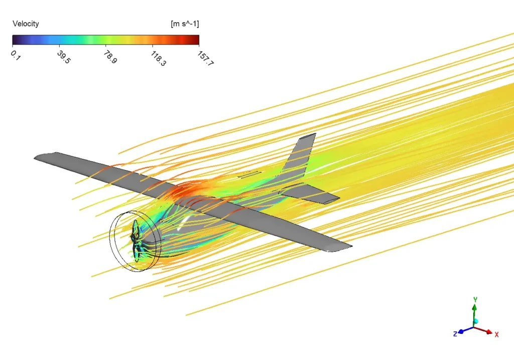
Figure 2: Flow analysis over a plane as a great example of CFD application in aerodynamics
Biomedical Applications
The biomedical field has embraced computational fluid dynamics for studying blood flow, respiratory systems, and drug delivery. CFD modeling helps medical researchers understand complex biological flows without invasive procedures.
Important biomedical applications include:
- Blood flow simulation in arteries, veins, and heart chambers
- Cardiovascular device design (artificial heart valves, stents, VADs)
- Respiratory airflow analysis in lungs and airways
- Drug delivery optimization through blood vessels or airways
- Medical device design for dialysis, oxygenation, and filtration
- Surgical planning and intervention simulation
- Biomechanical flow interactions with tissues
Explore our CFD in Biomedical Engineering collection to see how computational fluid dynamics simulation is advancing healthcare and medical technology.
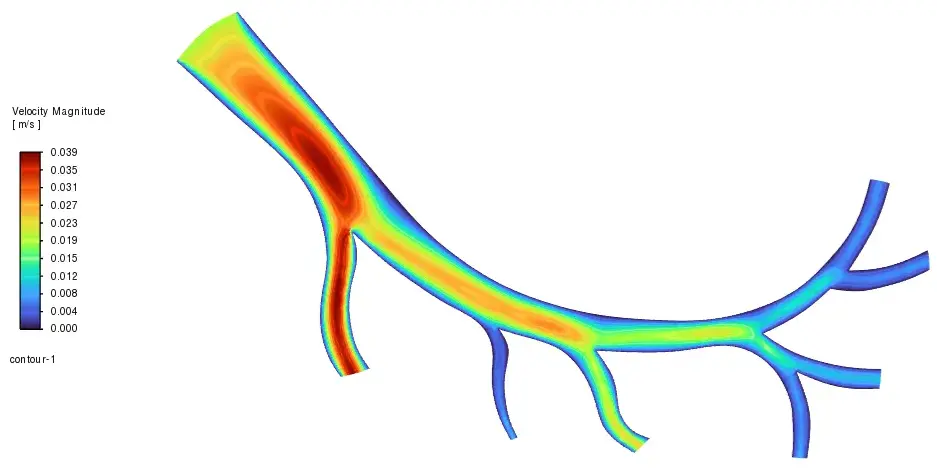
Figure 3: Blood flow CFD analysis in an artery vein
HVAC and Building Systems
Heating, ventilation, and air conditioning (HVAC) systems benefit tremendously from computational fluid dynamics analysis. Engineers use CFD programs to predict airflow patterns within buildings, optimize duct designs, and ensure proper ventilation throughout spaces.
Key HVAC applications include:
- Indoor air quality and ventilation effectiveness
- Thermal comfort analysis in occupied spaces
- Data center cooling optimization
- Natural ventilation design for buildings
- Contaminant dispersion and control
- Energy efficiency optimization for heating and cooling systems
- Smoke management for fire safety systems
Discover practical HVAC solutions in our HVAC CFD Simulation tutorial collection, where you can see real-world applications of computational fluid mechanics in building systems.
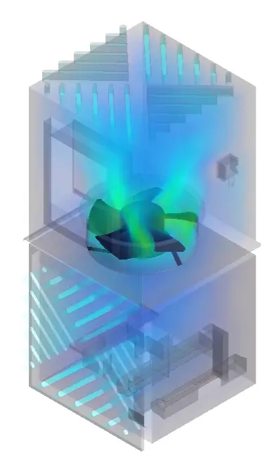
Figure 4: Air purifier design optimization for thermal comfort in an office
Renewable Energy Systems
The renewable energy sector increasingly relies on computational fluid dynamics to improve efficiency and reduce costs. From wind turbines to solar collectors, CFD simulation helps engineers optimize clean energy technologies.
Important renewable energy applications include:
- Wind turbine blade aerodynamics and farm layout optimization
- Solar collector thermal performance analysis
- Hydropower turbine design and efficiency improvement
- Wave and tidal energy converter optimization
- Geothermal system flow and heat transfer
- Biomass combustion process improvement
- Energy storage system thermal management
Browse our Renewable Energy CFD Simulation tutorials to see how computational fluid dynamics programs are accelerating the transition to sustainable energy.
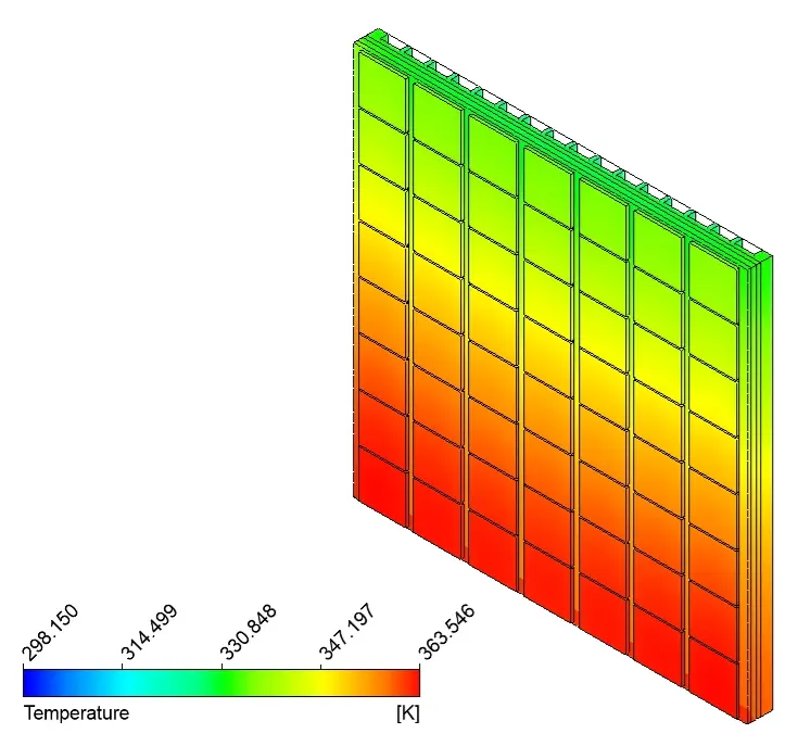
Figure 5: Thermal analysis of Solar panel
Automotive Industry
The automotive industry makes extensive use of computational fluid dynamics to improve vehicle design. CFD analysis helps create more aerodynamic, efficient, and comfortable vehicles while reducing development time and costs.
Key automotive applications include:
- External aerodynamics for reduced drag and improved fuel economy
- Engine cooling system optimization
- HVAC system design for passenger comfort
- Combustion process improvement in engines
- Exhaust system performance
- Battery thermal management for electric vehicles
- Noise reduction and acoustics
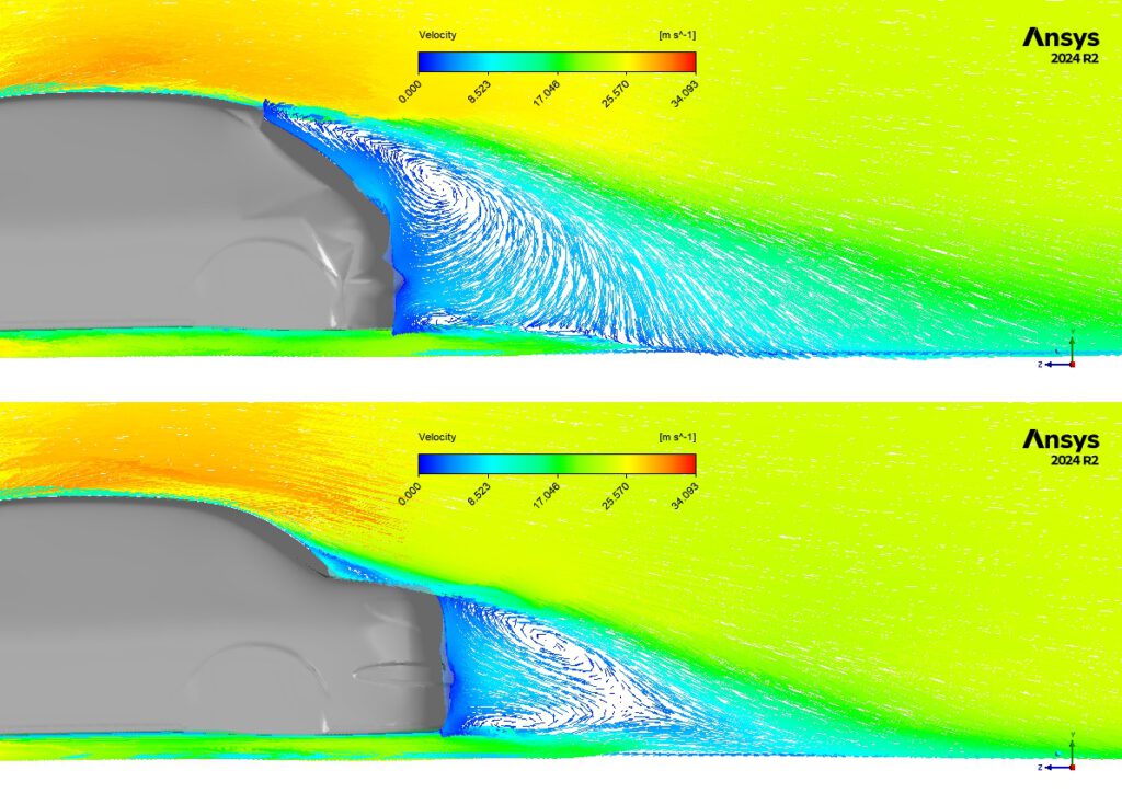
Figure 6: Aerodynamic performance of hatchback Vs. Sedan car
Environmental Engineering
Environmental engineers use computational fluid dynamics to address a wide range of challenges related to air, water, and soil quality. CFD modeling helps predict how pollutants disperse and develop effective remediation strategies.
Common environmental applications include:
- Urban air quality and pollution dispersion
- River and coastal flow modeling
- Wastewater treatment process optimization
- Groundwater flow and contaminant transport
- Weather pattern prediction
- Natural disaster impact assessment
- Climate change effects on local environments
Industrial Processes
Many manufacturing and process industries rely on computational fluid dynamics simulation to optimize their operations. CFD analysis improves efficiency, product quality, and safety across numerous industrial applications.
Key industrial applications include:
- Chemical reactor design and optimization
- Mixing and agitation process improvement
- Heat exchanger performance analysis
- Spray drying and coating processes
- Multiphase flow systems
- Filtration and separation equipment design
- Process safety analysis and hazard prevention
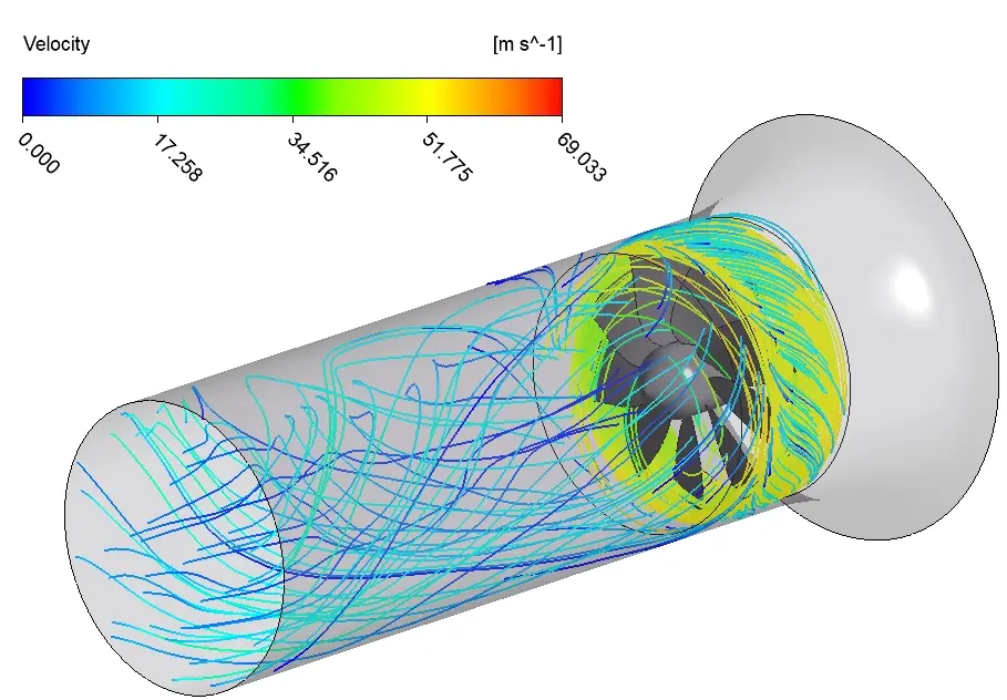
Figure 7: Fan design performance in a duct channel
From aerospace to renewable energy, computational fluid dynamics continues to transform how engineers solve complex problems across virtually every industry. The versatility and power of modern CFD software make it an indispensable tool for innovation and optimization in fields where fluid flow matters.
Computational Fluid Dynamics example
The lid-driven cavity flow is a classic benchmark problem in CFD used to study the behavior of fluid flow within a square or rectangular cavity. Engineers and researchers typically test their CFD models in this problem to assess the accuracy of their simulations. In other words, this example serves as a fundamental test case for CFD algorithms and is utilized to validate numerical methods and codes.
In simulating lid-driven cavity flow using Computational Fluid Dynamics, a rectangular cavity is defined with stationary walls on three sides and a lid moving at a constant velocity on the top. The governing equations, typically the Navier-Stokes equations for incompressible flow, are discretized using numerical methods like Finite Volume Method (FVM) or Finite Difference Method (FDM). The cavity is meshed, with a finer grid near the walls to capture boundary layer effects accurately. The simulation computes the velocity and pressure fields within the cavity iteratively until a steady-state or time-dependent solution is reached. Post-processing involves analyzing the flow patterns, shear stresses, and other relevant parameters to understand the behavior of fluid flow within the cavity.
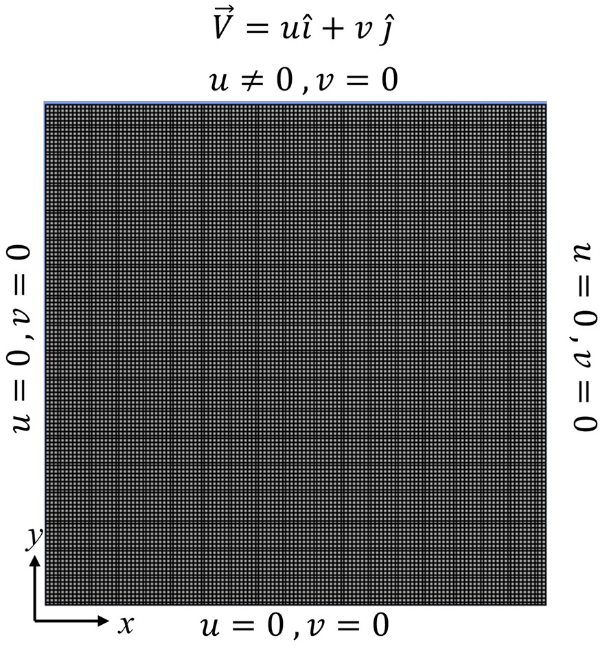
Figure 8: Meshed domain and boundary conditions of lid-driven cavity
ANSYS FLUENT Capabilities in Computational Fluid Dynamics
ANSYS Fluent is designed for CFD problems based on FVM. Within the ANSYS software suite, all aspects of CFD problem solving, including geometry definition, meshing, problem solving, and post-processing, are executed effectively. ANSYS Fluent possesses the capability to simulate highly intricate cases in CFD, encompassing combustion, multiphase flows, turbulent flows, and more. Moreover, the software can simultaneously simulate the mentioned cases, demonstrating its versatility and robustness in handling complex fluid dynamics scenarios.
At CFDLAND, we have completed numerous projects using ANSYS Fluent, all of which can be viewed in our CFDshop. Additionally, you can submit your CFD projects through the Order Project section. Trust our team of CFD experts to handle even the most complex simulations with proficiency and precision.
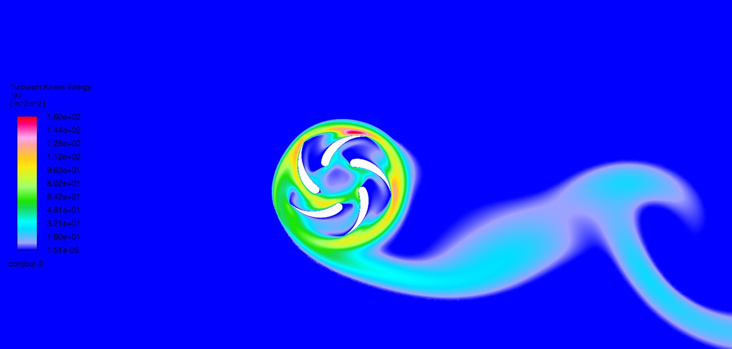
Figure 9: Turbulent kinetic energy contour based on ANSYS Fluent simulations from “5-blade Vertical Axis Wind Turbine CFD Simulation”
Conclusion
In an era defined by digital innovation, Computational Fluid Dynamics emerges as a transformative force in engineering. From its historical roots to contemporary applications, CFD’s evolution reflects a relentless pursuit of accuracy and efficiency. With ANSYS Fluent leading the charge, engineers navigate fluid dynamics complexities with confidence, driving advancements across industries. As CFD continues to push boundaries, its impact on design, optimization, and performance enhancement remains unmatched, shaping a future where fluid dynamics mastery fuels limitless innovation and progress.
Related Articles
- ANSYS for Student – Free CFD Software:Ready to start your computational fluid dynamics journey? Learn how students can access professional CFD simulation tools at no cost.
- Energy Conservation Equation: Understand one of the fundamental equations that powers all CFD analysis and discover how energy conservation principles are applied in computational fluid dynamics.
- Conservation of Mass in Fluid Mechanics: Explore the critical mass conservation principle that forms the foundation of all CFD modeling and ensures accurate fluid flow simulation results.
- CFD Applications: Discover the diverse industries where computational fluid dynamics solves complex engineering problems and see real-world examples of CFD simulation in action.