

Understanding y+ (y plus) in CFD is essential for simulating fluid velocity near solid walls. This dimensionless quantity helps you choose the right wall functions and create an accurate near-wall mesh. In this guide, we will learn the characteristics of the boundary layer, explain the law of the wall, and show how ANSYS Fluent handles these near-wall regions with high accuracy.
What is y+ (y plus) in CFD?
In a turbulent flow regime, the inertial forces are much higher than the viscous forces. However, the fluid velocity always drops near solid boundaries or walls. This happens because of the no-slip condition. The no-slip condition means that the fluid velocity on the solid surface is exactly zero. This assumption is not true everywhere, but it is highly accurate for most fluid mechanics problems.
Because the velocity drops at the wall, the inertial forces decrease. As a result, the viscous force becomes dominant in this near-wall region. This creates a very thin area next to the wall known as the boundary layer, where viscous effects control the flow. You must study and understand this area to simulate fluid flows accurately and choose the correct turbulence models.

Figure 1: The no-slip shear condition near the walls makes the flow velocity zero. This region is critical for Y-plus investigation
y+ Formula and Near-Wall Equations
To describe fluid flow near solid walls, we use two dimensionless quantities: u+ and y+. These are defined using the y+ formula and equation as follows:
[latexpage]
\[
u^+ = \frac{U}{u_t}=f \left( \frac{\rho u_ty}{\mu} \right)=f\left(y^+ \right)
\]
This relationship is known as the law of the wall. In this y+ equation, U is the velocity [m/s] at distance y from the wall [m], ut is the friction velocity [m/s], ρ is the fluid density [kg/m³], and μ is the dynamic viscosity [Pa·s].
[latexpage]
\[
u_t=\sqrt{{\frac{\tau_w}{\rho}}}
\]
Here, τw represents the wall shear stress [Pa]. Based on the y+ value, the boundary layer is divided into three distinct regions:
1. Linear or viscous sub-layer (y+ < 5)
In this region very close to the wall, the fluid velocity is low, and the viscous force is completely dominant. Because of this, it is called the viscous sub-layer. We assume the shear stress is constant and equal to the wall shear stress. This gives us:
[latexpage]
\[
\tau(y) = \mu \frac{\partial U}{\partial y}\cong \tau_w
\]
If we integrate this with respect to y and apply the boundary condition U=0 when y=0, we find a linear relationship between the mean velocity and the distance from the wall:
[latexpage]
\[
U = \frac{\tau_w y}{\mu}
\]
By using simple algebra and the definitions of u+ and y+, we get the final equation for this region:
[latexpage]
\[
u+=y+
\]
Because of this direct relationship, this area is also known as the linear sub-layer.
2. Buffer layer (5 < y+ < 30)
This layer sits between the viscous sub-layer and the log-law layer. Here, neither the inertial force nor the viscous force is entirely dominant; both are active. As a result, the velocity distribution is complex. CFD software handles the buffer layer using specific turbulence models and near-wall treatments. Simulation models often use damping functions or blending techniques to calculate the smooth transition of velocity from the viscous sub-layer up to the log-law region.
3. Log-law layer (30 < y+ < 300)
In this layer, both viscous and turbulent effects are important. The velocity distribution follows a logarithmic equation:
Because of the linear relationship between u+ and y+, this area is known as the linear sub-layer.
[latexpage]
\[
u+=\frac{1}{\kappa} \mathrm{ln} (y+)+B
\]
For standard flows, the von Kármán constant (κ) is 0.41, and B is an empirical constant, typically 5.15.
y+ graph
The following graph compares the equations presented in this article with experimental results (points). You can clearly see that these equations express the relationship between u+ and y+ very well. In this graph, the term (1/κ)ln(E)=B is used for the equation of the logarithmic region.
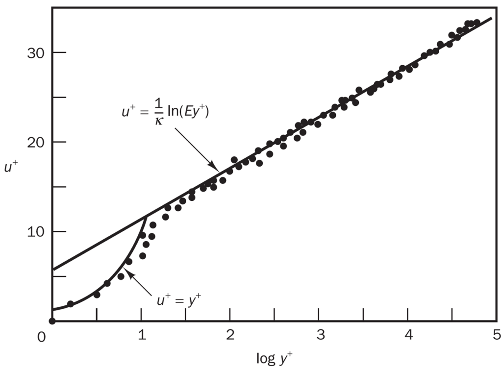
Figure 2: Velocity distribution near a solid wall. Adopted from “An Introduction to Computational Fluid Dynamics” by H K Versteeg et al.
Why Should y+ be Calculated in CFD Simulations?
Depending on which turbulence model you use and what your simulation goal is, your mesh resolution near the wall needs to have different sizes. One of the key parameters to determine this mesh resolution is the wall y+. You can easily calculate your required first cell height using our free y+ calculator.
Before running a simulation, you must know your target y+ based on your chosen turbulence model. This target dictates how you build the inflation layer, which we cover in detail in session 9 of our free ANSYS Meshing course. There are two main approaches for near-wall treatment:
- Wall functions approach: Compared to other methods, this method uses a coarser mesh, which reduces computational cost. It relies on the wall function y+ equations described earlier. However, it is less accurate for complex flows with flow separation or high pressure gradients. If you use this method, the center of the first mesh cell should sit at 30 < y+ < 300.
- Near-wall model approach (low-Reynolds number modeling): In this method, the viscous sublayer is directly resolved with a very fine mesh where the viscous force is dominant. This method provides proper accuracy in simulating complex flows and flow separation. To achieve high accuracy, this method requires y+ values of approximately 1 or less. While highly accurate, it demands higher computing power due to the small mesh size. This method is strongly recommended when your goal is to measure forces on walls.

Figure 3: This mesh resolution is suitable based on low-Reynolds number modeling. The velocity in the range of the red curve is calculated with this method.
Figure 4: This mesh resolution is suitable based on the wall functions approach. The velocity in the range of the red curve is calculated with this method.
k-ε vs k-ω SST & Target y+
Choosing the right y+ depends heavily on your selected turbulence models. The Standard k-ε (k-epsilon) model is excellent for simulating free stream flows, but it struggles to simulate the flow near solid walls accurately. Because of this, wall functions are usually used with the k-ε model.
On the other hand, the k-ω SST (Shear Stress Transport) model is famous for its high accuracy in simulating near-wall flows. To achieve maximum accuracy, the y+ for k-omega SST should be less than 1. Although larger y+ values can be used, this will reduce the accuracy of your results. After completing your CFD run, you must check the actual y+ on the walls. If the resulting y+ shows that your mesh resolution was incorrect, you will need to adjust your mesh and redo the simulation.
Worked Example: Forward y+ Calculation
To verify your mesh, you can perform a manual y+ calculation in the forward direction. In this example, a fluid (air at 20°C) flows over a flat surface. We will calculate the dimensionless wall distance using the y+ equation and the following parameters:
- Free-stream velocity (U∞): 10 m/s
- Plate length (L): 1 m
- Distance of first grid point from the wall (y): 0.0001 m
- Air density (ρ): 1.204 kg/m³
- Dynamic viscosity (μ): 1.825 × 10⁻⁵ kg/(m·s)
- Kinematic viscosity (ν = μ/ρ): 1.516 × 10⁻⁵ m²/s
First, we find the Reynolds number:
[latexpage]
\[
Re=\frac{\rho U_\infty L}{\mu}=\frac{1.204\times10\times1}{1.825\times 10^{-5}}=659726
\]
Next, we calculate the skin friction coefficient using the 1/7-power-law turbulent flat-plate correlation:
[latexpage]
\[
C_f=\frac{0.026}{Re^{1/7}}=\frac{0.026}{659726^{1/7}}=0.00383
\]
Then, we find the wall shear stress:
[latexpage]
\[
\tau_w = \frac{1}{2} C_f \rho U^2_\infty = 0.5 \times 0.00383 \times 1.024 \times 10^2=0.2308 \ \mathrm{Pa}
\]
The friction velocity is:
[latexpage]
\[
u_t=\sqrt{{\frac{\tau_w}{\rho}}} = \sqrt{\frac{0.2186}{1.204}}=0.4378 \ \mathrm{m/s}
\]
Finally, the y+ is:
[latexpage]
\[
y+ = \frac{u_t y}{\nu}=\frac{0.4261\times 10^{-4}}{1.516\times 10^{-5}}=2.89
\]
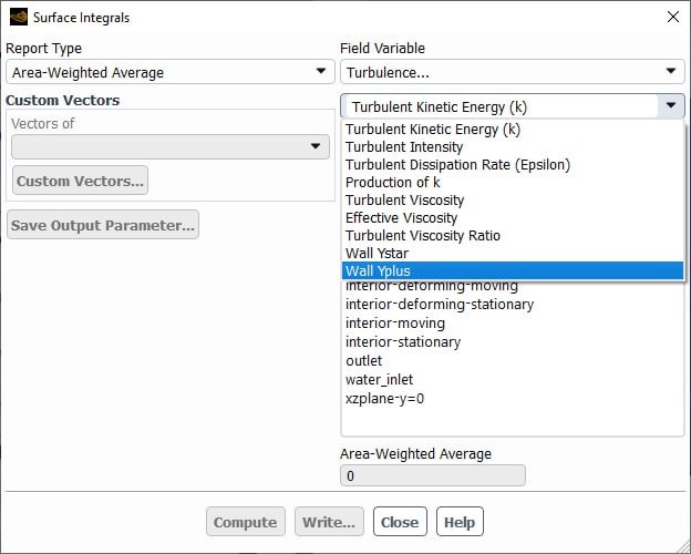
Figure 5: In ANSYS Fluent, in the surface integrals section, after simulation, you can extract the size of y+ on all boundaries and walls.
How to Check y+ in ANSYS Fluent
After running your simulation, you should verify the near-wall mesh resolution. Extracting the ANSYS Fluent y+ value is very simple. You can check the actual y+ fluent results directly in the software by following these steps:
- Go to the Results tab and click on Surface Integrals.
- Choose Area-Weighted Average or Facet Maximum from the report type drop-down.
- Under the Field Variable category, select Turbulence… and then choose Wall Yplus.
- Select your solid wall boundaries from the list.
- Click Compute to see the actual y+ value on those walls.
y+ Values for Different Turbulence Models in ANSYS Fluent
ANSYS Fluent handles the near-wall region, boundary layer, and wall functions exceptionally well. In all turbulence models, Fluent’s algorithms are highly advanced. Even if you do not design a perfect mesh, Fluent can often produce reasonable results. However, you should always follow the guidelines discussed in this article to achieve optimal accuracy.
As shown in the following figure, ANSYS Fluent simulates a wide range of viscous models. For each model, it provides detailed near-wall treatment options. You should base your selection on validated simulation work or past experience.

Figure 6: Viscous model settings panel stays here
Our experts at CFDLAND have completed numerous academic and industrial projects utilizing ANSYS Fluent for CFD simulations. They have a lot of experience in simulating near-wall fluid behavior and can validate results against previous simulations or experimental data. For assistance with your CFD projects, please visit our ORDER ANSYS Fluent Project page.
Conclusion
To study fluid flow near solid walls, we use the dimensionless quantity y+. This value helps us define wall functions, which accurately match experimental fluid behavior. Because y+ determines your near-wall mesh size, it is critical for setting up reliable turbulent flow simulations. While wall functions are great for many cases, complex flows require direct near-wall modeling.
Before setting up your next CFD mesh, you must know your target y+. Once you have that target, you can calculate your first cell height using our free tool to ensure your boundary layer is perfectly sized.
Frequently Asked Questions about y+
- What is a good y+ value? A good y+ value depends entirely on your chosen turbulence model and near-wall treatment. For the standard wall function approach, a y+ value in CFD between 30 and 300 is ideal. For near-wall modeling, you should target a y+ of 1 or less.
- Why should y+ be less than 1 for k-ω SST? The k-ω SST model is designed to resolve the thin viscous sublayer directly. To achieve the highest accuracy, the y+ for k-omega SST must be 1 or lower. This ensures the center of your first mesh cell is securely inside that viscous region.
- How do I check y+ after my simulation in ANSYS Fluent? You can easily check the y+ fluent results using the Surface Integrals tool under the Results tab. By selecting Wall Yplus from the Turbulence field variables, you can view the exact ansys fluent y+ on any boundary to verify your mesh.
- How do I calculate the first cell height for a target y+? Finding the physical wall distance from a target y+ requires a complex inverse calculation based on your fluid properties and Reynolds number. Instead of doing this manually, you should use an online calculator tool to find the exact height before meshing.
- Is a y+ check the same as a grid independence study? No. A y+ check only ensures your first mesh layer is sized correctly for your turbulence model. A grid independence test is a broader study to ensure that your overall simulation results do not change when you refine the entire mesh.
- What is the dimensionless wall distance? The dimensionless wall distance is simply another name for y+. It relates the physical distance from the wall to the local friction velocity and kinematic viscosity, allowing engineers to standardize boundary layer equations.