Setting DPM Boundary Conditions in ANSYS Fluent

When a simulation with discrete particles is run, the physical behavior of particles hitting a wall must be defined. Does the particle bounce off? Does it stick? Or does it simply disappear? The answers to these questions are controlled by DPM boundary conditions.

To achieve an accurate multiphase result, the particle-wall interaction must be correctly set. These boundary conditions tell the solver how a particle behaves when it reaches a surface zone. The choice made here completely changes the simulation results. In ANSYS Fluent, several types of particle boundary conditions are available, including:

• Reflect: The particle bounces off the wall.
• Trap: The particle gets stuck on the wall.
• Escape: The particle leaves the simulation domain.
• Wall-jet: The particle hits the wall and creates a thin stream of fluid.
• Wall-film: The particles form a liquid layer on the surface.

In this complete guide, each boundary condition is explained in simple. The function, the correct application, and the setup process are detailed for a successful simulation.

If you are interested in seeing practical examples and learning through prepared tutorials, we invite you to see our comprehensive DPM CFD simulation projects in the CFDLAND shop.

How to Set DPM Boundary Conditions in ANSYS Fluent

Before explaining what each condition does, the location of these settings in the software must be known. The particle-wall interaction can be set for any wall or boundary in the geometry.

Here are the basic steps that need to be followed:

1. In the Fluent setup tree, open the Boundary Conditions task page.
2. From the list, select the boundary zone you want to modify (for example, “wall-inlet-pipe”).
3. Click the Edit… button. A new window for that specific boundary will open.
4. In this new window, click on the DPM tab.

This DPM tab is where the particle behavior is controlled. A drop-down menu is provided where the particle boundary condition type can be chosen. The main options are Reflect, Trap, Escape, Wall-jet, and Wall-film.

Before we explain what each DPM boundary condition does, it is important to know where to find these settings in ANSYS Fluent. Luckily, the process is very simple. You can set the particle-wall interaction for any wall or boundary in your model.

Here are the basic steps you need to follow:

1. In the Fluent setup tree, go to the Boundary Conditions task page.
2. From the list, select the boundary zone you want to modify (for example, “wall-inlet-pipe”).
3. Click the Edit… button. This will open a new window for that specific boundary.
4. In this new window, click on the DPM tab.

This DPM tab is where you control everything that happens when a particle from the Discrete Phase Model hits that surface. You will see a drop-down menu where you can choose the particle boundary condition type. The main options you will find are Reflect, Trap, Escape, Wall-jet, and Wall-film.

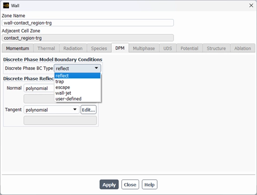
Figure 1: DPM Boundary condition tab in ANSYS Fluent

Exploring DPM Boundary Condition Types

The different types of wall interactions used in ANSYS Fluent are detailed below. The simplest and most common setting is Reflect.

Reflect: When Particles Bounce Off a Surface

The Reflect boundary condition is what it sounds like. When a particle hits a wall, it bounces off and continues its journey through the fluid domain. This is similar to a tennis ball hitting the ground. It is one of the most fundamental types of particle-wall interactions.

To control how the particle bounces, two important parameters must be defined: the coefficients of restitution. These coefficients are numbers between 0 and 1. They dictate how much momentum (or energy) the particle keeps after the collision.

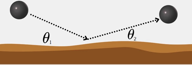
Figure 2: An illustration of the Reflect DPM boundary condition, where a particle hits a surface and bounces back into the flow domain, with its new path determined by the coefficients of restitution.

There are two coefficients that can be set:

• Normal Coefficient of Restitution: This controls the “bounce” in the direction perpendicular to the wall.
• Tangential Coefficient of Restitution: This controls the particle’s momentum parallel to the wall surface.

The chosen value is very important:

• A value of 1 means a perfectly elastic collision. The particle loses no momentum in that direction.
• A value of 0 means the particle loses all of its momentum in that direction after the collision.
• A value between 0 and 1 (e.g., 0.8) represents a real-world, inelastic collision where some energy is lost.

When to Use the Reflect Condition? This condition is applied in simulations where solid particles bounce off hard surfaces without sticking. For instance, in our tutorial on Magnetic Nanoparticles in an Artery, we simulate how nanoparticles travel through a blood vessel. For the artery walls, the Reflect condition is assigned because the particles are expected to bounce off the walls rather than stick to them.

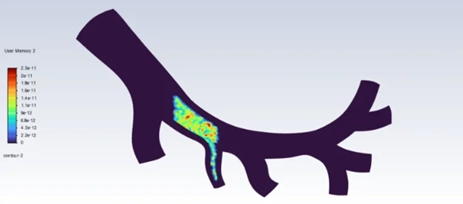
Figure 3: Nanoparticle bounce off after hitting the walls of artery

Trap DPM: When Particles Stick to a Surface

If particles need to be captured by a wall instead of bouncing off, the Trap DPM boundary condition is used. When a particle hits a surface with the Trap condition, the solver stops tracking its trajectory. The particle is considered “trapped” and is removed from the calculations.

This boundary condition is highly useful for engineering applications. The fate of the trapped particle’s mass depends on its material type:

• For solid particles (like sand or dust), they are simply removed from the calculation.
• For liquid droplets, their mass is instantly added to the surrounding gas as vapor.
• For combusting particles, any remaining volatile material is released into the cell.

The Trap condition is the standard choice for modeling filtration, deposition, or any process where particles stick to a solid surface. A classic application is a particle filter simulation. In our Particle Filtration DPM CFD Simulation tutorial, particles flow towards a filter mesh. The Trap boundary condition is used on the filter’s surface to accurately simulate the capture of the particles.

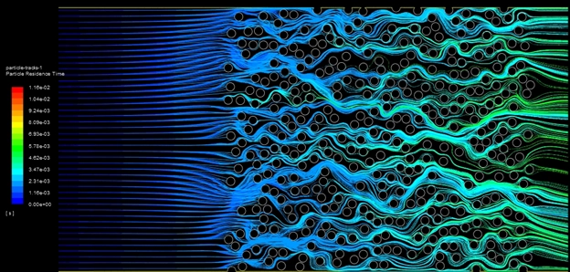
Figure 4: A CFD contour plot from a particle filtration simulation using the Trap DPM boundary condition. The colored particle tracks show how particles are captured by the filter surfaces.

Escape: When Particles Leave the Simulation

The Escape boundary condition is used when particles leave the simulation domain completely. Think of it like an open window in a room. If a dust particle flies out the window, it does not need to be tracked anymore. When a particle hits an Escape boundary, all calculations for that specific particle are stopped. The trajectory is terminated, and the particle is marked as “escaped” in the final report. Its mass is fully removed from the domain.

This is the required condition for outlets, vents, or any open boundary where particles naturally exit the system. Applying Escape correctly is simple but essential for defining a realistic physical model.

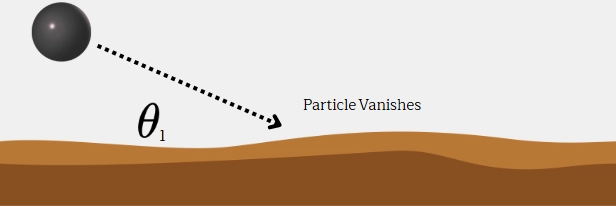
Figure 5: The ‘Escape’ condition allows the particle to pass through the boundary and exit the simulation domain, which is different from ‘Reflect’ or ‘Trap’.

Wall-jet: When a Droplet Splashes on a Surface

When a liquid droplet hits a wall, it might spread out and create a thin, fast-moving sheet of liquid. To model this behavior, the Wall-jet condition is used.

The Wall-jet boundary condition simulates a droplet hitting a wall and splashing outwards in a thin sheet, like a small “jet” moving along the surface. Think of throwing a water balloon at a wall; the water does not just stick, it splashes. This specific model is highly useful for high-temperature walls. On a very hot surface, a liquid droplet evaporates too quickly to form a stable film. Instead, it splashes across the heated metal.

The Wall-jet model is heavily used for liquid spray hitting hot surfaces, such as fuel spray inside a hot engine cylinder. The fuel droplets hit the hot piston walls and create a wall-jet. The behavior depends on physical factors like impact speed and impact angle.

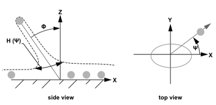
Figure 6: The Wall-jet DPM boundary condition simulates a droplet hitting a surface and splashing outward as a thin sheet, which is common for spray interacting with hot walls.

Wall-film: When Particles Form a Liquid Layer

The Wall-film model is one of the most powerful DPM boundary conditions available. It is essential for many advanced industrial simulations. This condition is used when liquid particles hit a surface and create a continuous liquid layer, or film. Instead of bouncing or escaping, the particles merge into this film. The solver then uses a separate set of equations to calculate how this liquid film moves, spreads, and evaporates on the surface.

Now we come to one of the most powerful and useful DPM boundary conditions in ANSYS Fluent: The Wall-film model. This model is essential for many advanced simulations.

The Wall-film DPM condition is used when you expect liquid particles to hit a surface and create a continuous liquid layer, or film. Instead of bouncing, getting trapped, or escaping, the particles merge with this film. The ANSYS Fluent DPM model then solves a separate set of equations to track how this film moves, spreads, and evaporates on the surface.

Figure 7: Liquid droplet after hitting a wall with Wall-film boundary condition [Lu, Kai, et al. “A study on urea deposition performance based on a new mixer design in diesel after-treatment system.” Chemical Engineering Research and Design 203 (2024): 731-741.]

This model handles complex physics. The outcome of a droplet hitting a wall-film depends on impact energy and wall temperature. The particle can:

• Stick/Spread: Join the film smoothly.
• Rebound: Bounce off the liquid film.
• Splash: Hit the film and cause smaller droplets to be ejected back into the fluid flow.

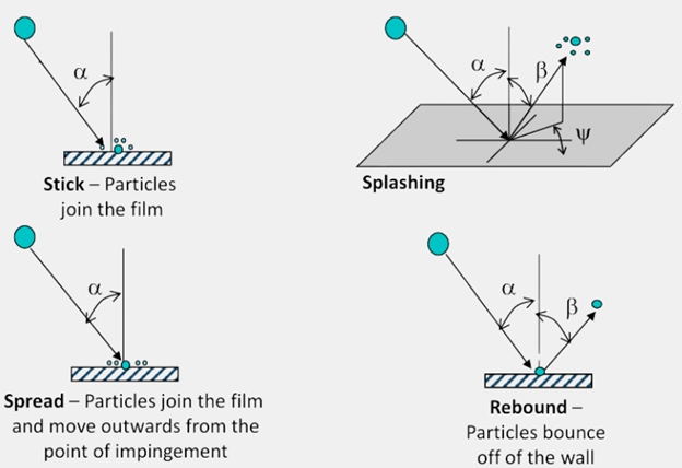
Figure 8: Droplet reaction after hitting a wall with wall-film DPM condition

The Wall-film model is critical for modeling spray cooling, film condensation, and surface icing. It requires an unsteady particle tracking setup and is strictly used for liquid droplets. A perfect example is our DPM Wall-film on a Heat Sink tutorial. In this simulation, a water spray cools a hot electronic component. The Wall-film condition is used on the heat sink surface to show how water droplets form a thin layer, which then evaporates to remove heat.

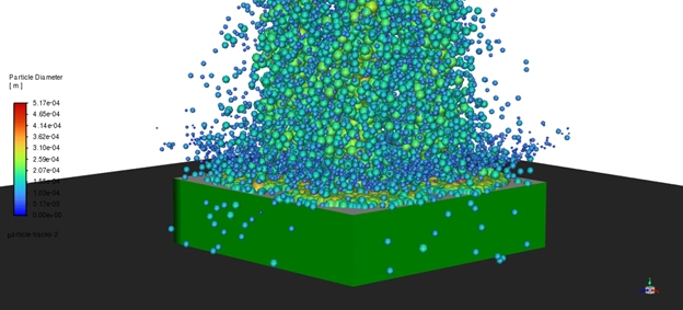
Figure 9: A CFD simulation result showing the formation of a liquid wall-film on a heat sink due to spray cooling, a key application of the Wall-film DPM boundary condition.

User-Defined: For Custom Interactions

Finally, a User-Defined boundary condition is offered. This is an advanced option used for highly specific engineering problems. It allows custom C-code, called a User-Defined Function (UDF), to be written to control exactly what happens when a particle hits a wall. This gives the engineer complete freedom. For example, a UDF can change a particle’s physical properties after a collision or trigger a surface chemical reaction. This is applied when standard models are not sufficient.

How to Choose the Right DPM Boundary Condition

Choosing the correct boundary condition is critical for generating valid simulation results. Each setting represents a different physical reality. To make the selection process simple, a comparison table is provided below.

Boundary Condition	What Happens to the Particle?	Best For…
Reflect	The particle bounces off the wall, like a ball. You set how much energy it loses.	Simulations where particles are solid and do not stick, like sandblasting or nanoparticles bouncing off artery walls.
Trap	The particle sticks to the wall and is removed from the simulation.	Filtration systems, particle deposition on surfaces, soot collection.
Escape	The particle leaves the simulation domain completely.	Outlets, vents, and open boundaries where particles exit the system.
Wall-jet	A liquid droplet hits a hot wall and splashes outward as a thin sheet.	Simulating spray hitting very hot surfaces, like in engine cylinders, where no stable film can form.
Wall-film	Liquid droplets hit a wall and form a continuous liquid film that can move and evaporate.	Spray cooling, icing simulations, fuel film on engine parts, condensation.
User-Defined	The particle’s fate is controlled by custom code (UDF) that you write.	Very complex or unique interactions not covered by standard models. Requires programming knowledge.

Conclusion

Defining suitable DPM boundary conditions is a major step in multiphase flow simulations. From a simple elastic bounce (Reflect) to a complex liquid layer (Wall-film), these settings dictate the physical validity of the particle-wall interaction. The correct choice between Reflect, Trap, Escape, Wall-jet, and Wall-film must be based on the actual physical phenomena expected in the system. Applying the right boundary condition transforms a basic visual model into a valuable, accurate engineering tool.

If you need professional assistance with your multiphase setup, you can review our DPM CFD Simulation Services category. Also, you can easily order your CFD project. The geometry and boundary settings will be reviewed to ensure your simulation is physically correct.