Boussinesq Approximation

The Boussinesq approximation is a widely used simplification in computational fluid dynamics (CFD) for modeling buoyancy-driven flows, particularly in natural convection problems. By assuming density variations are negligible except in the buoyancy term, the approximation simplifies the Navier-Stokes equations, reducing computational complexity while maintaining accuracy for small temperature differences. This paper explores the theoretical foundations of the Boussinesq approximation, and Additionally, the limitations of the Boussinesq hypothesis, particularly in cases where significant Boussinesq approximation density variations occur, are analyzed. The study provides insight into the relevance of the Boussinesq approximation in modern CFD simulations and its decreasing significance due to advancements in computational capabilities. A specific application of the Boussinesq approximation in ANSYS Fluent simulation is presented to highlight its practical implementation.

Types of Convection

Convection can be classified into two main types: natural convection and forced convection.

• Natural Convection: This occurs when fluid movement is driven by buoyant forces due to variations in density caused by temperature differences. No external force is involved in this process.
• Forced convection: when external sources such as fans and pumps are used for creating induced convection, it is known as forced convection

The Fig.1 illustrates the difference between forced convection and natural convection, showing how airflow is induced by a fan in forced convection, while in natural convection, air movement occurs due to buoyancy caused by temperature differences around a hot egg.

Figure 1- The cooling of a boiled egg by forced[1]

Buoyancy Force

In a gravitational field, there is a net force that pushes upward a light fluid placed in a heavier fluid. The upward force exerted by a fluid on a body completely or partially immersed in it is called the buoyancy force. The Fig.2 illustrates the concept of buoyancy using a simple object floating in water. The magnitude of the buoyancy force is equal to the weight of the fluid displaced by the body. That is,

Figure 2- Forces Acting on a Floating Object: Buoyancy vs. Weight[2]

Boussinesq Approximation

The Boussinesq approximation is a key simplification in fluid dynamics that facilitates the modeling of natural convection and buoyancy-driven flows. It is commonly used in CFD simulations to avoid solving the full compressible Navier-Stokes equations, thereby reducing computational costs. This approximation is particularly useful in applications where temperature-induced density variations are small, such as atmospheric circulation, ocean currents, and industrial heat transfer problems. The Boussinesq approximation assumes that density variations are negligible except in the buoyancy term of the momentum equation, where they drive flow due to gravitational forces.

Limitations of the Boussinesq Approximation

The Boussinesq approximation is a widely used simplification in fluid dynamics and CFD, but it comes with several limitations that restrict its applicability in certain scenarios:

Small Temperature Differences

It is only valid for small temperature variations (typically <10–20 K). Large temperature gradients lead to significant density changes, making the approximation inaccurate.

Incompressible Flow Assumption

The approximation treats the fluid as incompressible, which limits its application to low-speed flows. In compressible flows, where density variations influence the continuity equation and other governing equations, the Boussinesq approximation becomes invalid.

Modern Alternatives:

With advancements in computational power, solving the full compressible Navier-Stokes equations has become feasible, reducing the reliance on the Boussinesq approximation for high-accuracy simulations.

Overall, these limitations highlight that the Boussinesq approximation is best suited for small-scale, low-speed buoyancy-driven flows with minimal density variations.

Governing Equations: According to the Boussinesq Approximation

Under the Boussinesq approximation, the governing equations for mass, momentum, and energy are modified to account for the assumption of constant density except in the buoyancy term.

Continuity Equation (Mass Conservation):

If u is the local velocity of a parcel of fluid, the continuity equation for conservation of mass is:

This implies incompressible flow.

Momentum Equation (Navier-Stokes with Buoyancy Term):

The general expression for conservation of momentum of an incompressible, Newtonian fluid (the Navier–Stokes equations) is:

where µ is the kinematic viscosity,  is reference density, p is the pressure and g is the gravitational acceleration.

Using the Boussinesq approximation, density variations are small and modeled as:

Where:

rho= Local Density
rho_0= Reference Density
β = Coefficient of Thermal Expansion
T = Local Temperature
T_0= Reference Temperature

Substituting this in the momentum equation:

The change from p to P is referred to as a pressure shift.

Energy (Heat Transfer) Equation:

where  is the thermal diffusivity. Here, k is thermal conductivity, and  is specific heat capacity

Key Assumptions of the Boussinesq Approximation

• Density variations are neglected except in the buoyancy term
• The approximation is valid for small temperature differences where
• The flow remains incompressible.

Applications of Boussinesq Approximation

• Natural convection in enclosures (e.g., heated rooms, cooling of electronics).
• Atmospheric flows where temperature variations cause buoyancy-driven motions.
• Ocean currents and geophysical flows influenced by temperature gradients.

Boussinesq approximation CFD

When a fluid is heated, causing its density to change with temperature, gravity acts on these density variations, generating flow. These buoyancy-driven flows, known as natural convection (or mixed convection), can be simulated using ANSYS Fluent.

Modeling Natural Convection in a Closed Domain

When simulating natural convection within a closed domain, the solution is influenced by the mass inside the domain. Since the mass remains unknown without knowing the density, the flow must be modeled using one of the following approaches:

1. Conduct a transient simulation where the initial density is determined based on the initial pressure and temperature, ensuring that the initial mass is known. As the solution evolves over time, mass conservation is maintained. This approach is essential when significant temperature variations exist within the domain.
2. Use a steady-state simulation with the Boussinesq model, where a constant density is defined to ensure the mass is properly specified. This method is suitable only for cases with small temperature differences; for larger variations, a transient approach is required.

For instance, in CFDLAND shop, we explored the Natural convection in vertical cylindrical enclosures based on a valuable reference paper entitled “ Laminar natural convection in a laterally heated and upper cooled vertical cylindrical enclosure”. Our CFD model was successfully validated against the paper data which proves our knowledge over adoption of Boussinesq approximation and modeling natural convection.

Laminar Natural Convection In Cylindrical Enclosure CFD simulation, Numerical Paper Validation

Simulating the Buoyancy-Driven Flow in ANSYS Fluent

The following procedure outlines the steps for incorporating buoyancy forces when simulating mixed or natural convection flows.

Step1: Enable heat transfer calculations by selecting the Energy option in the Energy dialog box.

• Navigate to Models > Energy > Edit… to access the energy settings.

Step2: Set the operating conditions by configuring the parameters in the Operating Conditions dialog box (Fig.3).

• Go to Cell Zone Conditions > Operating Conditions… to define the operating parameters.

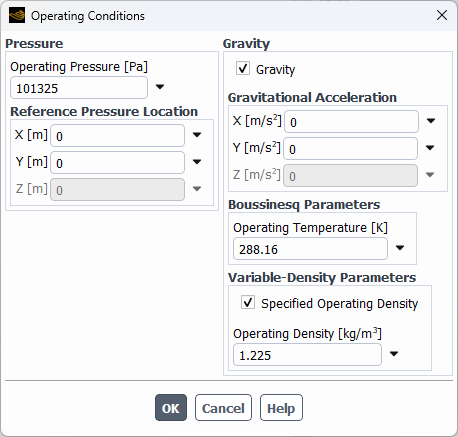
Figure 3- The Operating Conditions Dialog Box

• Enable the Gravity option in the Gravity
• Input the correct gravitational acceleration values for the X, Y, and (for 3D cases) Z directions (Keep in mind that ANSYS FLUENT sets the default gravitational acceleration to zero).
• If applying the incompressible ideal gas law, ensure the Operating Pressure is set to a suitable non-zero value.
• Enter the Operating Temperature ( ) in the Operating Conditions dialog box.

Step3: Set the Materials Properties

• In the Create/Edit Materials dialog box, select Boussinesq from the Density drop-down list, and specify a constant value (Fig.4).

 

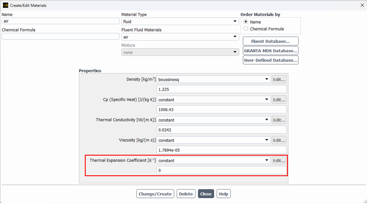
Figure 4- Thermal expansion coefficient in ANSYS Fluent

• In the Create/Edit Materials dialog box, specify a suitable value for the Thermal Expansion Coefficient (B ) for the fluid material.

Keep in mind that if your model includes multiple fluid materials, you can decide whether or not to apply the Boussinesq model to each material. Consequently, some materials may use the Boussinesq model while others do not. In such situations, you will need to configure all the parameters outlined in this step.

Step4: Solution Methods

• Choose either Body Force Weighted or Second Order from the drop-down list for Pressure under Spatial Discretization in the Solution Methods task page.
• If using the pressure-based solver, it is recommended to select PRESTO! as the Spatial Discretization method for Pressure.
• If needed, add cells near the walls to capture boundary layers effectively.

ANSYS Fluent Tutorial by Applying the Boussinesq Approximation

The Boussinesq Approximation plays a crucial role in simulating natural convection, where density variations are small but have significant effects on fluid motion. At CFD Land, we offer high-quality Boussinesq approximation CFD products that demonstrate the practical applications of this approximation. Our Natural Convection from Heat Sink Fins CFD Simulation, Numerical Paper Validation provides insights into cooling performance in electronic devices. The Natural Convection in a Narrow Annulus CFD Simulation, ANSYS Fluent Training is an excellent resource for learning and validating heat transfer in confined geometries. These products help engineers and researchers apply the Boussinesq Approximation effectively in their CFD analyses. Notice that! All are VALIDATION CFD simulations performed against valuable experimental & numerical papers.

Natural Convection In a Narrow Annulus CFD Simulation, ANSYS Fluent Training

Natural Convection From Heat Sink Fins CFD Simulation, Numerical Paper Validation

Conclusion

The Boussinesq approximation is a crucial simplification in computational fluid dynamics for modeling buoyancy-driven flows, particularly in natural convection problems, by assuming that density variations only affect the buoyancy term. While this approximation significantly reduces computational complexity, it is most effective in cases with small temperature differences. However, it has limitations, especially when dealing with large temperature gradients or compressible flows, where more advanced models are necessary. As computational power continues to improve, the need for such simplifications may decrease, but the Boussinesq approximation will remain relevant for many practical applications, providing accurate and efficient simulations in scenarios where its assumptions are valid.

FAQs

1. What is the Boussinesq approximation in CFD?

It’s a simplification in CFD where density variations are ignored except in the buoyancy term, used for natural convection with small temperature differences.

2. When is the Boussinesq approximation applicable?

It’s used in low-speed, incompressible flows with small temperature differences (less than 10–20 K) where density changes are minimal except for buoyancy.

3. What are the limitations of the Boussinesq approximation?

It doesn’t work well for large temperature gradients or compressible flows where density variations are significant throughout the fluid.

4. How does the Boussinesq approximation simplify CFD simulations?

By ignoring density variations except in the buoyancy term, it reduces the complexity of the Navier-Stokes equations, making simulations more efficient.

5. What are some real-world applications of the Boussinesq approximation?

It’s used in natural convection applications like electronic cooling, geophysical flows, and industrial heat transfer where temperature differences are small.

6. How do I apply the Boussinesq approximation in ANSYS Fluent?

In ANSYS Fluent, select the Boussinesq model in material properties and define the thermal expansion coefficient for the fluid.

Reference

[1]        A. J. Ghajar and Y. A. Cengel, ME 237: Heat and Mass Transfer; fundamental and applications. McGraw-Hill Education, 2015.