

Have you ever wondered why energy never disappears? Moreover, how do engineers use the energy conservation equation to design better systems? The law of conservation of energy is one of the most fundamental principles in physics and engineering. In simple words, the energy equation tells us that energy cannot be created or destroyed. Furthermore, it can only change from one form to another. For instance, when you heat water, electrical energy becomes thermal energy. Similarly, in CFD simulations, we track how energy moves through fluids. The conservation of energy equation helps engineers solve real problems. Additionally, it’s essential for designing HVAC systems, heat exchangers, and many other applications. In fact, without understanding the energy balance equation, modern engineering would be impossible!
Looking to master energy modeling in practice? Check out our comprehensive tutorials on HVAC CFD Simulation and Heat Transfer CFD Simulation. These hands-on tutorials show you exactly how to apply the energy conservation equation in real engineering projects!
Now, let’s explore the energy equation in detail. We’ll explain everything using simple words and examples!
What is the Energy Conservation Equation?
The energy conservation equation is very important in engineering. This equation works with two other equations called the Navier-Stokes equations and the continuity equation. Together, these three equations help us understand how fluids move and change temperature in CFD simulations. When we talk about the energy equation, we are talking about how energy moves and changes. Energy is what makes things work. For example, your car needs energy from fuel to move. Also, your body needs energy from food to function. In the same way, fluids need energy to flow and change temperature.
The conservation of energy is a basic rule in physics. This rule says that energy cannot disappear or appear from nowhere. Instead, energy only changes from one type to another type. This is exactly what the energy conservation equation helps us track.
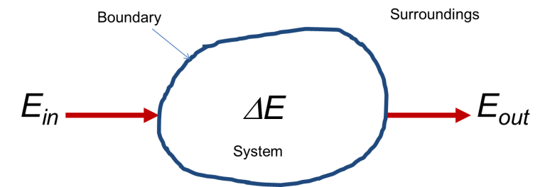
Figure 1: Energy conservation in a system
The energy balance equation can look different depending on what we are studying. For instance, when water turns to steam (we call this a phase change), the equation gets more complex. Also, when electricity is involved, we need to add more terms to the energy equation. However, the basic idea of energy conservation stays the same.
In fluid mechanics and CFD, solving the energy conservation equation can be hard. This is because we need to:
- Break down the equation into small parts (this is called discretizing)
- Connect the energy equation with other equations (this is called coupling)
- Solve many calculations quickly and accurately
Thankfully, a computer program called ANSYS Fluent helps engineers do these hard calculations. This software makes solving the energy equation much easier and faster.
In the next sections, we will also look at a simpler version of the energy equation called Bernoulli’s equation. This simpler equation is very useful in basic fluid mechanics problems.
The mathematical form of the energy conservation equation in its general form looks like this:

Where:
- E means the total energy per unit mass
- ρ means the fluid density
- v means the fluid velocity
- p means pressure
- k means how well heat moves through the fluid
- T means temperature
- S_h means any other energy sources
Understanding the energy conservation equation is essential for solving real engineering problems like heating, cooling, and fluid flow.
Energy Equation Derivation Made Simple
Have you ever wondered where the energy conservation equation comes from? In this section, we will learn the energy equation derivation in simple steps. Understanding how to derive the energy conservation equation helps us see why it works for so many different problems.
Starting Point: The First Law of Thermodynamics
To begin our energy equation derivation, we start with the First Law of Thermodynamics. This law simply states that energy cannot be created or destroyed, only transformed.
For a system, we can write this as:

Where:
- ΔE is the change in total energy
- Q is the heat added to the system
- W is the work done by the system
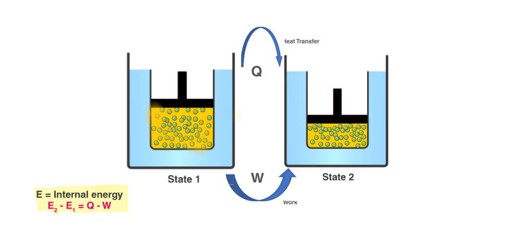
Figure 2: Energy conservation
This basic principle is the foundation for all forms of the energy conservation equation.
- Step 1: Consider a Small Fluid Element
To derive the energy conservation equation for fluids, we first look at a small box of fluid. This box has length Δx, width Δy, and height Δz.
The total energy in this box includes:
- Internal energy (heat)
- Kinetic energy (motion)
- Potential energy (height)
For each small fluid element, we track how energy enters, leaves, and changes over time.
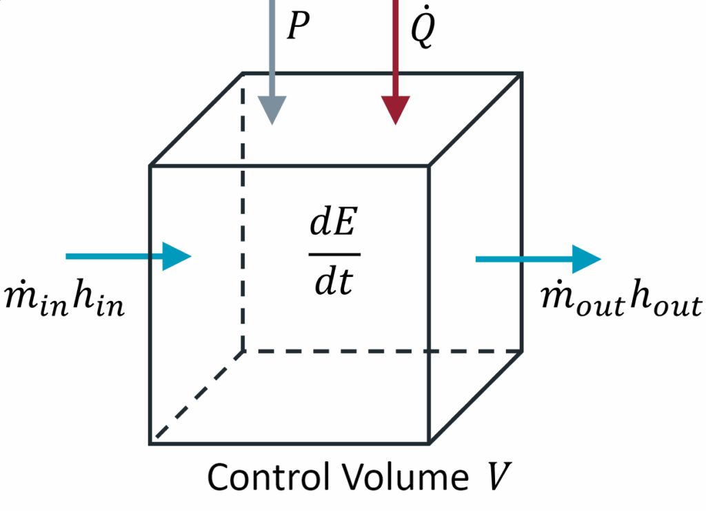
Figure 3 : Energy conservation in an control volume
- Step 2: Calculate Energy Flows
Now, we look at how energy moves in and out of our fluid box through its six faces. Energy can enter or leave by:
- Convection: Energy carried by the moving fluid
- Conduction: Heat flowing from hot to cold regions
- Work: Pressure forces doing work as fluid moves
- Sources: Any other energy generation inside the box
For example, the energy entering through the left face by convection is:

Where:
- ρ is density
- e is internal energy per unit mass
- P is pressure
- u is velocity in x-direction
Similar expressions can be written for all six faces of our fluid box.
- Step 3: Apply Conservation Principle
The energy conservation principle says that:
Rate of energy change = Net rate of energy in – Net rate of energy out + Net rate of energy generated
In mathematical form, this gives us:

Where:
- E is total energy per unit mass
- v is velocity vector
- P is pressure
- k is thermal conductivity
- T is temperature
- τ is stress tensor
- S_h is energy source term
This equation might look complex, but it simply states that energy must be conserved in every small region of the fluid.
- Step 4: Simplify for Specific Cases
The full energy equation can be simplified for specific cases. For example, for incompressible flow with constant properties, we can derive a simpler energy equation:

Where:
- c_p is specific heat
- Φ is viscous dissipation (friction heating)
This simpler form focuses just on temperature changes and is easier to solve for many engineering problems.
Knowing how to derive the energy conservation equation helps engineers:
- Choose the right form of the energy equation for their problem
- Understand the assumptions and limitations
- Know when to include or ignore certain terms
- Make appropriate simplifications for specific applications
The energy equation derivation is not just a mathematical exercise—it gives us powerful insights into how energy behaves in flowing fluids.
Energy Equation Forms: Differential vs Integral
The energy conservation equation can be written in two main mathematical forms: differential form and integral form. Each form has its own advantages and is useful in different situations. Let’s explore these forms and understand when to use each one.
Differential Form of Energy Conservation Equation
The differential form of the energy equation describes what happens at every tiny point in a fluid. It uses partial derivatives to show how energy changes with position and time.
The general energy conservation equation differential form looks like this:

Where:
- ρ is density
- E is total energy per unit mass
- t is time
- v is velocity vector
- p is pressure
- k is thermal conductivity
- T is temperature
- τ is stress tensor
- S_h is source term
This differential form is what CFD software like ANSYS Fluent solves using numerical methods.
The differential form is especially useful when:
- You need detailed information at specific points in the flow
- You are doing computer simulations
- You want to see how energy varies continuously through space
However, the differential form can be complicated to solve by hand, so we often use it with computer programs.
Integral Form of Energy Conservation Equation
The integral form of the energy equation looks at the total energy in a whole region rather than at individual points. It’s like looking at the big picture instead of tiny details.
The integral form of the energy conservation equation is:

Where:
- V is the volume region
- S is the surface of that region
- n is the unit normal vector to the surface
This form tells us how energy flows into and out of a specific region and how it changes inside that region.
The integral form is particularly useful when:
- You are interested in overall energy balance rather than point-by-point details
- You are doing hand calculations for engineering problems
- You want to analyze a specific component or region
Steady Flow Energy Equation
One important simplified version is the steady flow energy equation. “Steady” means conditions don’t change with time. This simplification is very useful in many engineering applications.
The steady flow energy equation in differential form looks like:

Notice that the time-dependent term is gone.
For practical engineering problems, we often use an even simpler steady flow energy equation between two points 1 and 2:

Where:
- h is enthalpy per unit mass
- v is velocity
- g is gravity
- z is height
- q is heat added per unit mass
- w is work done per unit mass
This simple form of the steady flow energy equation is extremely useful for analyzing systems like turbines, pumps, and heat exchangers.
Energy Equation in ANSYS Fluent
ANSYS Fluent is one of the most popular software programs for CFD simulations. It solves the energy conservation equation automatically when you turn on the energy model. Understanding how ANSYS Fluent handles the energy equation will help you set up more accurate simulations.
How to Enable the Energy Equation in ANSYS Fluent
Turning on the energy equation in ANSYS Fluent is simple. Here are the steps:
- Open your ANSYS Fluent project
- Go to the “Models” menu
- Click on “Energy”
- Check the box that says “Energy Equation”
- Click “OK”
That’s it! Now ANSYS Fluent will solve the energy conservation equation along with other flow equations. This simple step is essential for any heat transfer or temperature-dependent simulation.

Figure 2: To check the energy equation and temperature changes in ANSYS Fluent, go to the Setup menu, then to Models, and enable the energy equation.
Energy Equation Boundary Conditions in ANSYS Fluent
For the energy equation to work correctly, you must set the right boundary conditions. Boundary conditions tell the software what happens to energy at the edges of your model.
Here are the most common energy equation boundary conditions in ANSYS Fluent:
-
Temperature: You set a fixed temperature at a boundary. For example, a wall might be kept at 300 K.
-
Heat Flux: You specify how much heat flows through a boundary. The heat flux might be constant or vary with position.
-
Convective Heat Transfer: You define the surrounding temperature and a heat transfer coefficient. The heat transfer depends on the temperature difference.
-
Radiation: The boundary exchanges heat with surroundings through radiation.
The mathematical form for these boundary conditions might look like:


Choosing the right boundary conditions is crucial for getting accurate temperature predictions in your CFD simulations.
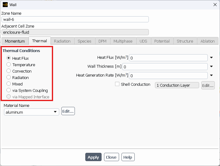
Figure 3: Energy boundary conditions panel in ANSYS Fluent
In CFDSHOP, you can view many of our completed projects in the field of CFD using ANSYS Fluent, indicating the capabilities of our experts. You can place your CFD project orders through ORDER CFD PROJECT, where our experts will handle even the most complex simulations.
ANSYS Fluent Energy Equation Forms
ANSYS Fluent adapts the energy equation based on your simulation type. Here are some ways the energy equation changes:
-
For incompressible flows (when density doesn’t change much), Fluent solves a simpler form focused on temperature.
-
For compressible flows (like high-speed air), Fluent solves the full energy conservation equation including pressure effects.
-
When you have multiphase flows (like water and air together), Fluent tracks energy in each phase separately.
-
For reacting flows (with chemical reactions), Fluent includes energy release or absorption from reactions.
This automatic adjustment means you don’t need to choose which energy equation form to use – ANSYS Fluent does it for you!
Energy Conversion Equation Example
As shown in the figure below, the air passes through the 700 hp turbine. Find the flow exit velocity and the heat transferred for the conditions indicated. (R = 1716, Cp = 6003 ft.lbf/(slug.°R))

Assuming a perfect gas, the fluid density at the inlet and outlet is:
![\[ \rho_1 = \frac{p_1}{RT_1}=\frac{150(144)}{1716(460+300)}=0.0166 \ slug/ft^3 \]](https://cfdland.com/wp-content/ql-cache/quicklatex.com-6e383fd5bbb6a5fb64adb36a45411194_l3.png "Rendered by QuickLaTeX.com")
![\[ \rho_2 = \frac{p_2}{RT_2}=\frac{40(144)}{1716(460+35)}=0.00679 \ slug/ft^3 \]](https://cfdland.com/wp-content/ql-cache/quicklatex.com-93e820b523f33e0ed03309aae056cb65_l3.png "Rendered by QuickLaTeX.com")
Inlet mass flow rate:
![\[ \dot{m} = \rho_1 A_1 V_1 = (0.0166)\frac{\pi}{4}(\frac{6}{12})^2(100)=0.325 \ slug/s \]](https://cfdland.com/wp-content/ql-cache/quicklatex.com-a12250caf37ddbba80a62c9e02127080_l3.png "Rendered by QuickLaTeX.com")
Knowing mass flow, we compute the exit velocity:
![\[ \dot{m} = 0.325 = \rho_2 A_2 V_2 = (0.00679)\frac{\pi}{4} (\frac{6}{12})^2 V_2\Rightarrow V_2=244 \ ft/s \]](https://cfdland.com/wp-content/ql-cache/quicklatex.com-f47c1eb4a3ed4a06eb96c3e9c729c324_l3.png "Rendered by QuickLaTeX.com")
Under steady state conditions, considering only the work of the shaft (Turbile), and defining the combination of internal energy and pressure terms as enthalpy (h = CpT), the energy equation is as follows:
![\[ \dot{Q}-\dot{W}_s = \dot{m}(C_p T_2 + \frac{1}{2} V_2^2 - C_pT_1 - \frac{1}{2} V_1^2) \]](https://cfdland.com/wp-content/ql-cache/quicklatex.com-37b04e9115c016754d82ff6adc43f249_l3.png "Rendered by QuickLaTeX.com")
![\[ 1 \ hp = 550 \ ft.lbf/s\Rightarrow \dot{W}_s=700(550) = 385000 \ ft.lbf/s \]](https://cfdland.com/wp-content/ql-cache/quicklatex.com-1f0df301961113d83a1f910cd705bf28_l3.png "Rendered by QuickLaTeX.com")
![\[ \dot{Q}-385000 = 0.325 [6003(495)+\frac{1}{2}(244)^2 - 6003(760) - \frac{1}{2} (100)^2 ] = -510000 \ ft.lbf/s\Rightarrow \dot{Q} = -125000 \ ft.lbf/s \]](https://cfdland.com/wp-content/ql-cache/quicklatex.com-086ef98e202d7a58c220dc0d78ab9ad3_l3.png "Rendered by QuickLaTeX.com")
![\[ \dot{Q} = -125000 \ ft.lbf/s \ \frac{3600 \ s/h}{778.2 \ ft.lbf/Btu} = -578000 \ Btu/h \]](https://cfdland.com/wp-content/ql-cache/quicklatex.com-53ce9ee2cd3c6a946461e53477bd9a5c_l3.png "Rendered by QuickLaTeX.com")
Types of Energy Conservation Equations in CFD
There are many different forms of the energy conservation equation that we use in CFD simulations. Each form helps us solve specific types of problems. Let’s look at the most important types of energy equations that engineers use.
Total Energy Equation
The total energy equation is the most complete form. This equation includes all types of energy in a fluid system. When we talk about total energy, we mean the sum of internal energy, kinetic energy, and potential energy.
In CFD, the total energy equation looks like this:

Where:
- e_t means the total energy per unit mass
- ρ means the fluid density
- v means the fluid velocity
- k means thermal conductivity
- T means temperature
- τ means stress tensor
- S_h means energy source terms
Internal Energy Equation
Sometimes, we only care about the internal energy (or heat) of the fluid. In this case, we use the internal energy equation. This form of the energy conservation equation focuses on temperature changes.

Where:
- e is the internal energy per unit mass
- Φ is the dissipation function (turning motion into heat)
Thermal Energy Equation
For many heat transfer problems, we use the thermal energy equation. This simplified form of the energy conservation principle focuses on how temperature changes in fluids.

Where:
- c_p is the specific heat capacity
- T is temperature
Enthalpy Form of Energy Equation
In systems with heat transfer and changing pressure, the enthalpy form of the energy equation is very useful. Enthalpy combines internal energy and pressure-volume work.

Where:
- h is enthalpy per unit mass
Choosing the right form of the energy conservation equation is critical for accurate CFD simulations. The choice depends on your specific problem and which energy effects are most important.
In ANSYS Fluent, you don’t need to worry about selecting the exact mathematical form. Instead, you select the physics models you need, and the software automatically uses the appropriate energy equation form for your simulation.
Bernoulli’s Equation: Simplified Energy Conservation
Bernoulli’s equation is a special, simplified version of the energy conservation equation. It was created by a scientist named Daniel Bernoulli in the 1700s. This equation is extremely useful because it makes energy conservation much easier to understand and apply for many everyday fluid flow problems.
What is Bernoulli’s Equation?
Bernoulli’s equation connects pressure, velocity, and height in a flowing fluid. In simple words, it tells us that when a fluid flows faster, its pressure decreases. Also, when a fluid gains height, it loses pressure. The Bernoulli equation is actually an example of mechanical energy conservation. This means it only looks at mechanical forms of energy – not heat or other types.
Here is how we write Bernoulli’s equation:

Where:
- P is the pressure
- ρ is the fluid density
- v is the fluid velocity
- g is gravity (9.81 m/s²)
- h is the height
Each term in the Bernoulli equation represents a different type of energy per unit volume:
- P is pressure energy
- ½ρv² is kinetic energy (energy of motion)
- ρgh is potential energy (energy of height)
When Can We Use Bernoulli’s Equation?
The Bernoulli equation is a simplified form of the energy conservation equation, so it only works under certain conditions:
- The fluid must be incompressible (not changing density)
- The flow must be steady (not changing with time)
- The flow must be frictionless (no viscous effects)
- The flow must be along a streamline
In real life, these conditions are rarely perfect. However, the Bernoulli equation still gives good results for many engineering problems. This is why the Bernoulli equation is so popular in fluid mechanics!
Real-Life Examples of Bernoulli’s Equation
Bernoulli’s principle explains many things we see every day:
- Airplane wings: The air moves faster over the top of the wing, creating lower pressure and lifting the plane.
- Spray bottles: Squeezing the bulb makes air move fast across a tube, lowering pressure and drawing liquid up.
- Baseball curve ball: The spinning ball creates different air speeds on different sides, causing pressure differences that curve the ball.
These examples show how mechanical energy conservation through Bernoulli’s equation helps us understand everyday phenomena.
How Bernoulli’s Equation Connects to the Full Energy Equation
The full energy conservation equation accounts for many effects that Bernoulli’s equation ignores, such as:
- Heat transfer
- Friction losses
- Unsteady flow
- Compressibility
However, when these effects are small, Bernoulli’s equation gives us a much simpler way to solve problems using energy conservation principles. This makes it an excellent starting point before moving to the more complex energy equations in CFD.
Conclusion: Why Energy Conservation Equations Matter
Throughout this article, we have explored the energy conservation equation in detail. This fundamental principle helps engineers solve countless problems in fluid mechanics, heat transfer, and many other fields.
The energy equation comes in many forms. We looked at:
- The general energy conservation equation for all situations
- Bernoulli’s equation as a simplified version for specific cases
- Different types of energy equations used in CFD
- How to implement the energy equation in ANSYS Fluent
- Real-world examples and applications of energy conservation
- The derivation of the energy equation in simple steps
- Both differential and integral forms of the energy conservation equation
Understanding the energy balance equation is essential for anyone working with fluids or heat transfer. Moreover, this knowledge forms the foundation for more advanced topics in engineering and physics.
When you use CFD simulations, the software solves these energy equations automatically. However, knowing what happens behind the scenes helps you set up better simulations and interpret the results correctly.
Whether you’re designing a heat exchanger, analyzing a cooling system, or studying aerodynamics, the conservation of energy principle will be at the core of your work.
Related Blogs
-
Convective Heat Transfer: Learn about convective heat transfer, which is a critical mechanism for energy transport that appears in many terms of the energy conservation equation.
-
Overall Heat Transfer Coefficient: Discover how the overall heat transfer coefficient affects energy transfer across boundaries, an essential concept when applying the energy equation to real-world heat exchangers.
-
Conservation of Mass in Fluid Mechanics: Understand the conservation of mass principle that works alongside the energy conservation equation as part of the fundamental conservation equations in fluid dynamics.
-
The Essential Fluid Dynamics Equations: Explore the complete set of fluid dynamics equations that includes the energy equation as one of its crucial components.
-
ANSYS Fluent Boundary Conditions: Master how to set proper boundary conditions in ANSYS Fluent for accurately solving the energy equation in your CFD simulations.