Incompressible vs. Compressible Flow

Ali Abbaspur
Reading time: 14 min

In fluid dynamics, understanding the distinction between compressible and incompressible flow is essential for solving engineering problems, analyzing fluid behavior, and designing efficient systems. Incompressible flows are those in which variations in density are negligible—commonly applicable to liquids—while compressible flows, typically involving gases, experience significant density changes. These differences directly impact the incompressible/compressible flow equations, relevant Mach number classifications, and required boundary conditions, particularly in CFD simulations using tools like ANSYS Fluent. This blog explores key concepts including compressible flow regimes, the role of Mach number in identifying flow type, and how fluid properties influence modeling choices. It also provides practical insight into applying these principles in CFD to improve simulation accuracy and optimize engineering designs.

Contents

Compressible vs. Incompressible Flow

A flow is classified as being compressible or incompressible, depending on the level of variation of density during flow. Incompressibility is an approximation, in which the flow is said to be incompressible if the density remains nearly constant throughout (Fig.1). Therefore, the volume of every portion of fluid remains unchanged over the course of its motion when the flow is approximated as incompressible.

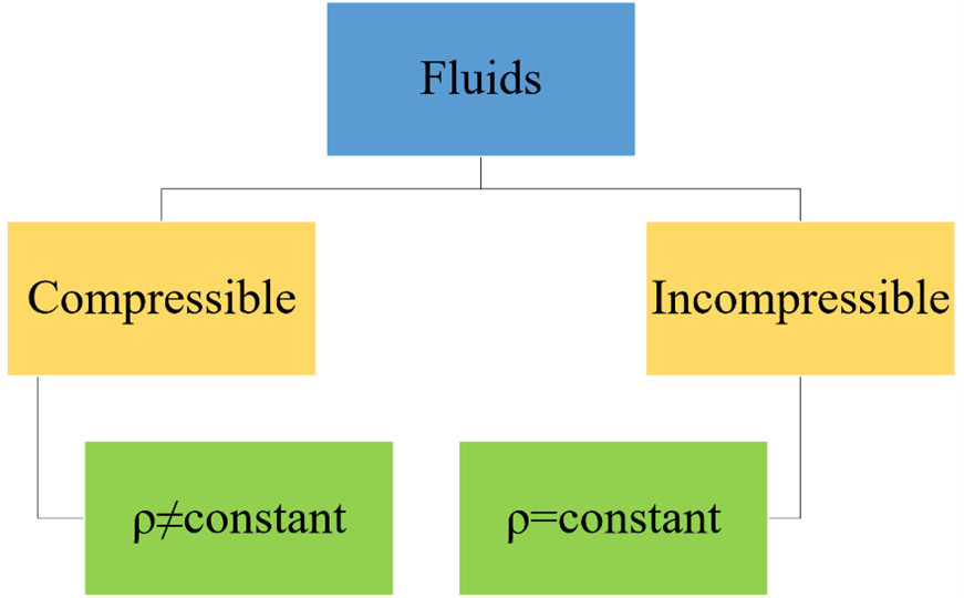
Figure 1- Compressible vs. incompressible flow different from density variation perspective

The densities of liquids are essentially constant, and thus the flow of liquids is typically incompressible. Therefore, liquids are usually referred to as incompressible substances. A pressure of 210 atm, for example, causes the density of liquid water at 1 atm to change by just 1 percent. Gases, on the other hand, are highly compressible. Compressible flow deals with fluids where density changes significantly within the flow field. This is common in gases moving at high velocities where pressure and temperature variations cause density changes. A pressure change of just 0.01 atm, for example, causes a change of 1 percent in the density of atmospheric air.

Our compressible CFD tutorial, “Energy Loss in Nozzle (Compressible Flow) CFD Simulation“, is based on the study “Numerical Analysis of Nozzles’ Energy Loss Based on Fluent (Fig.2).” This tutorial investigates how compressible flow through a nozzle leads to energy loss due to sharp pressure and velocity changes. Using ANSYS Fluent, the simulation highlights how nozzle geometry—such as inlet and outlet diameters and taper angle—impacts energy efficiency. It’s a valuable case study for engineers aiming to reduce losses in high-speed applications like water jets, rocket engines, or industrial sprayers.

Figure 2- Energy loss in nozzle CFD Simulation: Compressible flows tutorial with ANSYS Fluent

Incompressible and Compressible Example

To understand what is meant by this, imagine a fluid that fills a container that has one freely moving wall (Fig.3). The freely moving wall is pushed down by some mass. If the fluid is compressible, more mass pushing down on the freely moving wall will cause the particles of the fluid to move closer together, increasing its density. The following diagram shows this.

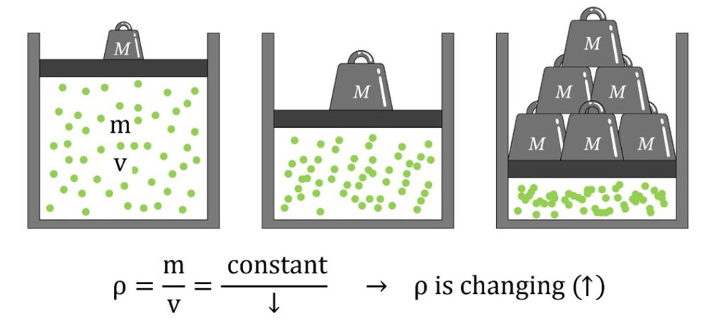
Figure 3- When density variations are not negligible, the fluid is called compressible.

If the fluid is incompressible, no matter how much mass is placed on the freely moving wall, the particles of fluid will not move closer together; the density of the fluid will not change (Fig.4). In other words, density is constant in an incompressible flow, and it is common for liquids such as water and oil to be considered incompressible fluids. This is illustrated in the following diagram.

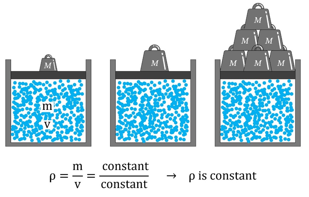
Figure 4- Fluid in which variations in density are negligible are termed incompressible.

Incompressible vs. Compressible Flow Equations

In computational fluid dynamics (CFD), the mathematical models used to simulate fluid behavior depend heavily on whether the flow is compressible or incompressible. The key difference lies in how density (ρ) is treated within the governing equations.

Table1 clearly highlights the fundamental differences between incompressible and compressible flow by comparing their governing equations. In incompressible flow, density is assumed constant, simplifying the continuity equation to a divergence-free velocity field, and eliminating the need for an equation of state. In contrast, compressible flow accounts for density variations, requiring more complex forms of the continuity, momentum, and energy equations, and introducing a thermodynamic relationship (e.g., ideal gas law) to close the system.

The momentum equation in compressible flow includes additional terms to capture density-driven effects, while the energy equation tracks changes in both internal and kinetic energy. These differences are especially important in CFD simulations, where choosing the correct flow model (compressible or incompressible) directly affects accuracy, especially in high-speed gas flows or when using tools like ANSYS Fluent.

Table 1- Comparison of Governing Equations for Incompressible and Compressible Flow

Equation Type	Incompressible Flow	Compressible Flow
Continuity	$\nabla \cdot \vec{V} = 0$	$\frac{\partial \rho}{\partial t} + \nabla \cdot (\rho\vec{V}) = 0$
Momentum	$\rho \left( \frac{\partial\vec{V}}{\partial t} + \vec{V} \cdot \nabla\vec{V} \right) = -\nabla p + \mu \nabla^2\vec{V} + \vec{F}$	$\frac{\partial(\rho\vec{V})}{\partial t} + \nabla \cdot (\rho\vec{V} \otimes \vec{V}) = -\nabla p + \nabla \cdot \boldsymbol{\tau} + \rho\vec{F}$
Energy	$\rho c_p \left( \frac{\partial T}{\partial t} + \vec{V} \cdot \nabla T \right) = k\nabla^2 T + \Phi$	$\frac{\partial(\rho E)}{\partial t} + \nabla \cdot [\vec{V}(\rho E + p)] = \nabla \cdot (k\nabla T) + \Phi$
State Equation	$\text{Not needed (constant }\rho\text{)}$	$p = \rho RT \text{ (ideal gas law or other EOS)}$
Viscous Stress Tensor	$\text{Often simplified: }\mu\nabla^2\vec{V}$	$\boldsymbol{\tau} = \mu \left(\nabla\vec{V} + (\nabla\vec{V})^T\right) - \frac{2}{3}\mu(\nabla \cdot \vec{V})\mathbf{I}$

One of our tutorials explores compressible flow behavior inside an ejector-diffuser system, where high-speed jets generate suction and pressure recovery without moving parts (Fig.5). Using ANSYS Fluent, the simulation captures key phenomena such as shock waves, flow mixing, and energy transfer between primary and secondary flows. The ejector’s converging-diverging geometry creates supersonic and subsonic regions that significantly affect pressure and temperature profiles. This tutorial, inspired by a reference study from the International Journal of Heat and Mass Transfer, demonstrates how CFD tools reveal complex flow interactions in cooling systems, propulsion devices, and vacuum generation setups.

Figure 5- CFD Simulation of fluid flow in ejector-diffuser system: Compressible flows tutorial with ANSYS Fluent

Role of Mach Number in Incompressible and Compressible Flow

Compressibility effect in a fluid flow can be obtained with Mach number. Mach number is a dimensionless number representing the ratio of flow velocity to sound velocity and expressing the level of density change caused by a flow:

$Ma = \frac{v}{c} = \frac{\text{Speed of flow}}{\text{Speed of sound}}$

where c is the speed of sound whose value is 346 m/s in air at room temperature at sea level. A flow is called sonic when Ma = 1, subsonic when Ma < 1, supersonic when Ma > 1, and hypersonic when Ma ≫ 1 (Fig.6).

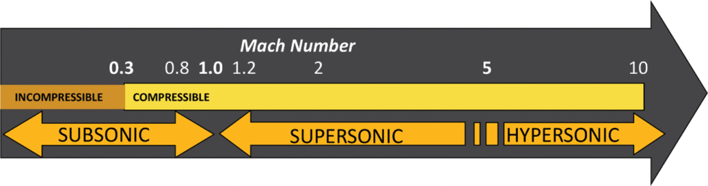
Figure 6- Flow regimes ranges based on Mach number

Liquid flows are incompressible to a high level of accuracy, but the level of variation of density in gas flows and the consequent level of approximation made when modeling gas flows as incompressible depends on the Mach number. Gas flows can often be approximated as incompressible if the density changes are under about 5 percent, which is usually the case when Ma < 0.3. Therefore, the compressibility effects of air at room temperature can be neglected at speeds under about 100 m/s.

At CFDLAND there is a free CFD tutorial focuses on transonic compressible flow over a 3D NACA0012 airfoil, analyzing the complex aerodynamic behavior around Mach 0.8 (Fig.7). Transonic regimes feature both subsonic and supersonic zones, making shock wave formation and pressure variation key aspects of this study. Using ANSYS Fluent, the simulation is based on a compressible air model with ideal gas assumptions, a 4° angle of attack, and a structured mesh. The pressure-based solver with compressibility effects (ideal gas + Sutherland model) provides sufficient accuracy for this case. The tutorial helps users understand how compressible effects influence drag, lift, and aerodynamic performance in realistic design scenarios.

Figure 7- Transonic Flow Over 3D NACA0012: Compressible flows tutorial with ANSYS Fluent

Small density changes of liquids corresponding to large pressure changes can still have important consequences. The irritating “water hammer” in a water pipe, for example, is caused by the vibrations of the pipe generated by the reflection of pressure waves following the sudden closing of the valves (Fig.8).

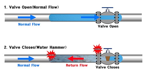
Figure 8- Water hammer phenomenon in a water pipe due to Small density changes of liquids

Although all gas flows are technically compressible, compressibility effects become noticeable primarily under certain conditions—such as when flow velocities are high and there are significant changes in pressure and density. However, if the Mach number is below approximately 0.3, the flow can generally be treated as incompressible, even for gases. This assumption simplifies the analysis considerably.

If you are still confused for distinguishing between incompressible and compressible flow, the Table 2 provides a clear comparison between incompressible and compressible flow based on key criteria such as Mach number, density variation, fluid type, and CFD modeling approach.

Table 2- Criteria for Identifying Incompressible vs. Compressible Flow

Criteria	Incompressible Flow	Compressible Flow
Mach Number	Mach < 0.3	Mach > 0.3
Density Variation	Negligible (assumed constant)	Significant (varies with pressure and temperature)
Pressure Ratio	Small pressure differences	Large pressure differences
Temperature Effects	Negligible influence on density	Strong influence on density
Fluid Type	Liquids, low-speed gases	High-speed gases

Incompressible vs. Compressible Flow in ANSYS Fluent

When setting up a compressible/ Incompressible flow simulation in ANSYS Fluent, it’s important to consider the following key points to ensure accurate and stable results:

Solver Selection

Fig.9 illustrates how the choice of solver in ANSYS Fluent depends on the Mach number and the nature of the flow. When Mach < 0.3, the flow is typically treated as incompressible, since density variations are negligible. At Mach = 0.3, compressibility effects may begin to appear, and for Mach > 0.3, the flow is considered compressible due to significant changes in density. Accordingly, pressure-based solvers are generally used for incompressible and low-speed compressible flows, while the pressure-based coupled solver can handle moderate compressibility. For high-speed compressible flows, especially those involving shocks or rapid density changes, the density-based solver is recommended for accurate and stable simulations.

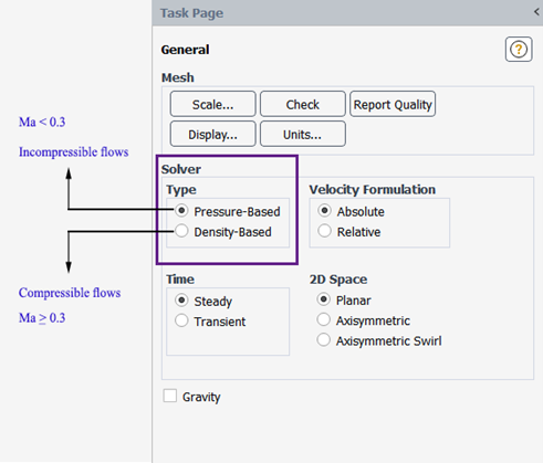
Figure 9- Guidelines for Choosing Between Pressure-Based and Density-Based Solvers in ANSYS Fluent

Enable Energy Equation

When setting up a compressible flow simulation in ANSYS Fluent, activating the energy equation (Fig.10) is essential because compressible flows inherently involve significant variations in temperature, pressure, and internal energy. These variables are strongly interdependent: changes in pressure affect temperature, which in turn alters fluid density and speed of sound. The energy equation accounts for these interactions by solving for thermal energy transport, including convection, conduction, and viscous dissipation. Without the energy equation, these key thermal effects would be ignored, leading to inaccurate predictions of flow behavior—especially in high-speed regimes where compressibility effects dominate.

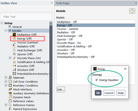
Figure 10- The energy equation must be activated for compressible flow simulation in ANSYS Fluent.

Density Models in ANSYS Fluent

Fig.11 displays the material property settings in ANSYS Fluent, where defining density behavior is crucial for accurate flow simulation. For incompressible flows, especially at low Mach numbers (Mach < 0.3), density is constant in an incompressible flow, as variations in pressure and temperature are minimal. Even when using an ideal-gas model, a gas can be treated as incompressible if the flow speed is low and thermal effects are negligible.

In contrast, compressible flow simulations require a variable density model, such as ideal-gas, to account for significant changes in pressure, temperature, and density. This setup is essential for high-speed flows where compressibility effects dominate. Selecting the correct density model in Fluent directly influences solver behavior and ensures accurate representation of fluid dynamics in different flow regimes.

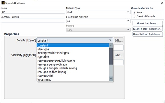
Figure 11- The schematic of material property selection for compressible/ incompressible of gas flows in ANSYS Fluent

Moreover, you can see the Boussinesq approximation which is a useful simplification applied in incompressible flow simulations with natural convection. It assumes that density is constant everywhere except in the buoyancy term of the momentum equation, where it is treated as a linear function of temperature. This allows you to capture the effects of temperature-driven flow (like warm fluid rising and cool fluid sinking) without fully modeling compressible flow behavior.

Boundary Conditions

When setting up compressible flow simulations in ANSYS Fluent, boundary conditions must account for the variable density effects. Unlike incompressible flows, at a pressure inlet, you are required to define both the gauge total pressure (also known as stagnation pressure) and the supersonic/initial gauge pressure (representing static pressure). Additionally, temperature input—typically total (stagnation) temperature—is needed to fully describe the thermodynamic state of the flow at the inlet. These values help Fluent compute the correct inlet conditions based on compressible flow theory. The Fig.12 shows how these fields are configured in Fluent.

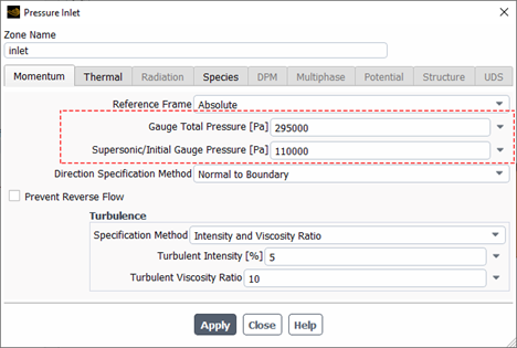
Figure 12- Pressure inlet boundary setup for compressible flow in ANSYS Fluent

A special boundary condition (called pressure far field in ANSYS-FLUENT) is also available for compressible flows (Fig.13). With this boundary condition, we specify the Mach number, the static pressure, and the temperature; it can be applied to both inlets and outlets and is well suited for supersonic external flows.

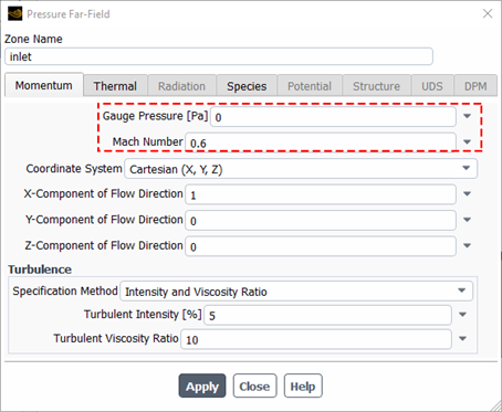
Figure 13- Pressure far field setting in ANSYS Fluent

Compressibility Effects in Turbulent Flow Simulation

Compressibility effects in turbulent simulations are essential for accurately capturing the influence of density variations caused by pressure and temperature changes, which are critical in high-speed flows such as supersonic and hypersonic regimes, where phenomena like shock waves, expansion regions, and aerodynamic heating significantly impact the overall flow behavior. Hence, enabling Viscous Heating and Compressibility Effects is crucial for accurately simulating high-speed compressible flows (Fig.14).

The Viscous Heating option accounts for the conversion of kinetic energy into thermal energy due to viscous friction in the fluid. This effect becomes significant in high-speed flows, especially in compressible regimes like supersonic or hypersonic flows, where temperature gradients can strongly affect density and flow properties. Neglecting this feature can lead to inaccurate predictions of thermal behavior, particularly in cases involving high shear rates or boundary layers.

The Compressibility Effects option modifies the turbulence model to account for density variations caused by pressure and temperature changes in compressible flows. This is essential for accurately modeling shock waves, expansion regions, and other phenomena that occur in flows with Mach numbers greater than 0.3. Without enabling compressibility effects, the turbulence calculations may incorrectly assume constant density, leading to errors in pressure, velocity, and temperature predictions. Together, these options ensure the fidelity of simulations for compressible flow regimes.

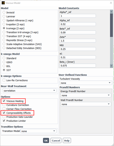
Figure 14- The importance of activating the compressibility effects in turbulent flow simulation

Shock Wave in Supersonic Flow CFD simulation is another CFDLAND product (Fig.15) which focuses on shock wave formation around the NACA0012 airfoil at Mach 1.5 and 4° angle of attack, highlighting key features of compressible flow at high speeds. Using ANSYS Fluent, the tutorial captures bow shocks, oblique shocks, and expansion waves, which dramatically affect pressure, temperature, and density fields. These phenomena strongly influence lift and drag, making them critical for aerospace design. As covered in Session 8 of our Fluent course, this tutorial provides a practical look at how shock waves behave in supersonic regimes and how CFD tools are used to analyze and optimize such flows.

Figure 15- Shock wave in supersonic flow CFD Simulation: Compressible flows tutorial with ANSYS Fluent

Conclusion

Understanding the difference between incompressible and compressible flow is crucial in fluid mechanics and CFD modeling. In incompressible flow, the density is assumed constant, simplifying the governing equations, especially when the Mach number is below 0.3. In contrast, compressible flow requires consideration of density variations, energy equations, and often complex flow regimes including subsonic, transonic, supersonic, and hypersonic. In ANSYS Fluent, choosing between pressure-based or density-based solvers depends on the compressibility of the flow. Furthermore, boundary conditions for compressible flows demand special attention—such as specifying stagnation properties. Mastering the right assumptions and solvers ensures accurate simulation results for both compressible and incompressible flows.

FAQs

Is density constant in incompressible flow?

Yes. In incompressible flow, the density is assumed constant, which simplifies the governing equations and is typically valid when the Mach number is less than 0.3.

What is the key difference between compressible and incompressible flow equations?

Compressible flow equations include density as a variable and require solving the energy equation, while incompressible flow equations assume constant density, often ignoring energy variations unless temperature effects are important.

At what Mach number does flow become compressible?

Flow is considered compressible when the Mach number exceeds 0.3, because density changes can no longer be neglected.

Why is the energy equation important in compressible flow simulations?

In compressible flow, temperature, pressure, and density are interrelated. Activating the energy equation in ANSYS Fluent allows proper modeling of these thermodynamic changes and energy losses.

Which solver should I use in ANSYS Fluent for compressible flow?

Use the density-based solver for high-speed, highly compressible flows. For moderate compressibility, the pressure-based coupled solver is often sufficient.

How are boundary conditions different for compressible flows in ANSYS Fluent?

For compressible flow boundary conditions, especially at inlets, you must define stagnation pressure, static pressure, and total temperature to accurately model the flow behavior.

How turbulent flow is handled in compressible/incompressible CFD simulations?

Turbulent flow in both compressible and incompressible fluid simulations is modeled using turbulence models like k-ε, k-ω SST, or LES. In compressible flows, additional care (activating Viscous Heating Compressibility Effects) is needed to ensure the turbulence model accounts for energy dissipation and shock-boundary interactions.