Interphase Forces in Eulerian Model: Drag and Non-Drag Forces

Kiarash Kord
Reading time: 19 min

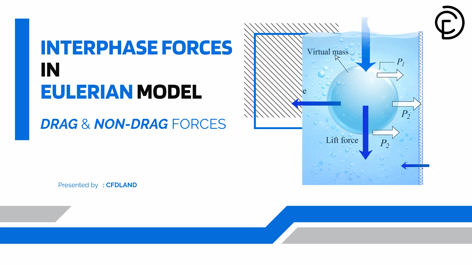
In our previous guide, Introduction to Eulerian Multiphase Model in ANSYS Fluent, we explained how the software uses conservation equations for different phases. Now, we must understand how these phases physically push and pull each other.

Contents

When gas bubbles rise in water, or solid particles move in air, they touch the surrounding fluid. The fluid and the particles share speed and energy. This connection is called interphase momentum exchange. In the Eulerian multiphase model, the software must calculate the exact forces acting on the secondary phase. If you choose the wrong force models, your multiphase flow simulation will completely fail. These forces control the bubble movement, the gas holdup, and the final physical results. If you want to see how we apply these settings in realistic industrial projects, you can review our professional Multiphase CFD Simulation tutorials.

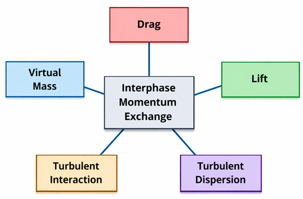
Figure 1: Block diagram showing the main components of interphase momentum exchange in the Eulerian multiphase model.

Overview of Interphase Forces

In ANSYS Fluent multiphase setups, we divide the momentum exchange into two main groups. We have the primary drag force CFD models, and we have several important non-drag forces. Here is a simple overview of the forces we will explain in this blog:

Drag Force: This is the main hydrodynamic friction between the continuous liquid and the dispersed bubbles. It is the most important force in any gas-liquid flow CFD project.
Lift Force: When the liquid velocity changes, this force pushes bubbles sideways.
Wall Lubrication Force: This is a special force that prevents bubbles from touching the solid walls of a pipe or tank.
Virtual Mass Force: When a bubble suddenly speeds up, it must push the heavy liquid around it. This creates an extra resistance force.
Turbulent Dispersion Force: This force happens when turbulent eddies hit the bubbles. It mixes the bubbles and spreads them out evenly.

In the next sections, we will explain exactly how each force works and how to set them up correctly.

Figure 2: All forces acting on a bubble in a water column

Buoyancy in Multiphase Flows

Before we look at complex drag forces, we must talk about the most basic force: buoyancy. In any multiphase flow simulation, gravity is always present. Gravity pulls all fluids down. But why do air bubbles go up? They go up because of buoyancy.

Gravity and Hydrostatic Pressure

If you have a tall tank of water, the water at the bottom has a higher pressure than the water at the top. We call this hydrostatic pressure. It happens because gravity pulls the water mass down. In the Eulerian multiphase model, the pressure gradient and the gravity force balance each other in the exact same equations. When you turn on gravity in ANSYS Fluent, the software automatically calculates this hydrostatic pressure for you.

Figure 3: Schematic of Hydrostatic pressure

Density Differences Between Phases

Buoyancy happens when two phases have different densities. For example, water is heavy, and air is very light. The density of liquid water is about 1000 times higher than the density of air. Because water is much heavier, gravity pulls the water down very strongly. The heavy water then pushes the light air bubbles up. This density difference creates a strong upward buoyancy force on the secondary phase. You can read more about Buoyancy and its principles in our unique blog here.

If you want correct phase interaction ANSYS Fluent results, you must always turn on the gravity setting. If you forget to turn on gravity, the bubbles will not rise, and your buoyancy multiphase flow calculation will fail completely. You can see how we set up gravity and buoyancy correctly in our ready Multiphase CFD Simulation tutorials.

Drag Force: Fundamentals

The drag force is the most basic and common force in fluid dynamics. You can think of drag as the hydrodynamic friction between the continuous liquid phase and the dispersed bubbles. When a bubble moves through water, the water pushes back against it. This resistance is the drag force. The drag force is the most important force in any gas-liquid flow CFD, and you must always include it in your Eulerian multiphase model setup.

To calculate the drag force, ANSYS Fluent uses a number called the drag coefficient (Cd). This number changes depending on the shape and size of the bubble. It also depends on the slip velocity, which is the speed difference between the moving water and the moving bubble. A fast, large bubble will have a very different drag coefficient than a slow, small bubble.

If you have only one bubble in a tank, you calculate the single bubble drag. However, in industrial pipes or reactors, you have thousands of bubbles moving together. We call this a bubble swarm. When bubbles move in a group, they affect the water around each other. The drag on a group of bubbles is very different from the drag on one bubble. Because of this, ANSYS Fluent calculates a special bubble swarm drag. The software multiplies the drag force by the gas volume fraction to get the correct physical result.

Interfacial Area Density: To find the total drag force CFD value in a computational cell, the software must know the total surface area of all the bubbles inside that cell. We call this the interfacial area density. For simple spherical bubbles, the software calculates the interfacial area density using the volume fraction and the bubble diameter ( $(A_i = 6\alpha/d_p)$ ). If you do not define the bubble diameter correctly, the interfacial area density will be wrong, and the total drag force will fail.

Figure 4: Diagram showing the basic concept of drag force acting as hydrodynamic resistance on a single bubble.

Bubble Shape and Flow Regimes

To calculate the correct drag force, we must know the exact shape of the bubbles. Bubble shapes change depending on their size, speed, and the fluid around them. Engineers use three important dimensionless numbers to find the correct shape:

Eotvos number (Eo): This number compares the buoyancy force with the surface tension force. It tells us the volume and shape of the bubble.
Morton number (Mo): This number looks at the physical properties of the fluids. It is constant for a specific fluid pair. For example, the Morton number for air and water is always 7.5e-11 .
Reynolds number for bubbles: This number compares the inertial forces with the viscous (friction) forces.

We use the Eotvos, Morton, and Reynolds numbers to draw a bubble regime map. This map shows three main bubble shape regimes:

Viscous regime (Spherical bubbles): When bubbles are small (around 1 mm in water), they are perfect spheres. They rise in a straight or zig-zag path.
Distorted regime (Ellipsoidal bubbles): When bubbles grow bigger, they become flat like an egg.
Cap regime (Spherical cap bubbles): When bubbles are very large (around 18 mm in water), they look like a mushroom cap or an umbrella.

The drag coefficient changes completely when a bubble moves from the viscous regime to the cap regime. In the cap regime, the drag coefficient reaches a constant value.

Figure 5: Bubble regime map showing spherical, ellipsoidal, and spherical cap bubble shapes based on Eotvos and Reynolds numbers.

*** In ANSYS Fluent, you do not need to guess the shape. The automatic flow regime detection Fluent tool calculates the drag for all shapes and automatically chooses the correct shape for your flow. It does this by checking the continuity of the drag coefficient.

Drag Models for Gas-Liquid Flows

In ANSYS Fluent, you cannot use one simple number for the drag coefficient. You must choose a specific mathematical model. The software uses these models to calculate the drag force automatically. We will explain the most important drag models for gas-liquid flow CFD, their governing equations, and exactly when you must use them in your simulation.

Figure 6: Drag laws available in Forces tab of Eulerian multiphase model in ANSYS Fluent

Schiller-Naumann model

The model is the oldest and most basic drag model. It assumes the bubble is a perfect hard sphere. The governing equation for this model is

$C_D = \frac{24}{Re} (1 + 0.15 Re^{0.687})$

when the Reynolds number (Re) is less than 1000. If the Reynolds number is higher than 1000, the drag coefficient becomes a constant value of . Also, if the bubble moves very slowly and the Reynolds number is less than 1, this equation simply becomes Stokes Law, which is

$C_D = \frac{24}{Re}.$

You must use the Schiller-Naumann model when you have small, constant, and perfect spherical bubbles that are smaller than 1 millimeter. Do not use it for large bubbles.

Morsi-Alexander model – Symmetric

It is very similar to the Schiller-Naumann model, but you must use it when you have a much larger range of Reynolds numbers. Another option is the Symmetric drag model. The Symmetric model uses the exact same Schiller-Naumann equation, but it calculates the fluid density and viscosity from the volume-averaged mixture properties. You must use the Symmetric drag model when the phases mix so much that the liquid becomes the secondary phase and the gas becomes the primary phase. This model is very good for phase inversion.

Grace drag law

When bubbles grow, they are not perfect spheres. They become flat or look like a mushroom. For these cases, you must use the Grace drag law. The Grace model calculates the drag for three different shapes, which are viscous, distorted, and cap shapes. It uses the Eotvos number and the Morton number in its governing equations. For very large cap bubbles, the governing equation becomes very simple, and the drag coefficient is exactly

$C_D = \frac{8}{3}$

You must use the Grace drag law when you have variable bubble sizes and tall bubble columns. The Grace model is highly recommended because it accurately calculates the terminal rise velocity for large, non-spherical bubbles in any multiphase flow simulation.

Tomiyama drag model

Another very smart choice is the Tomiyama drag model. This model looks at the actual shape of the bubble to find the correct drag force. Its governing equation calculates the drag for all three shapes at the same time and mathematically selects the correct one. The governing equation is

$C_D = \max(\min(C_{D,viscous}, C_{D,distorted}), C_{D,cap})$

You must use the Tomiyama drag model when you have many different bubble shapes in the same tank. It is the best model for flows where bubbles change shape quickly.

Universal drag law or the Ishii drag model

In very dense flows, bubbles hit each other and pack together. For these dense flows, you must use the Universal drag law or the Ishii drag model. Their governing equations use the gas volume fraction to change the drag coefficient. For example, in the Universal model, the fluid viscosity is mathematically divided by the gas volume fraction to show that the fluid acts thicker. You must use the Universal or Ishii models when you have dense bubbly flows. If your gas volume fraction is very high, you must use these dense models in your Eulerian multiphase model setup to account for the bubble swarm effect.

Lift Force

In many pipes and tanks, the water does not move at the same speed everywhere. When the liquid flow is not uniform or has rotation, bubbles feel a strong side push. This side push is called the lift force. Lift forces are very important because they change the radial distribution of the secondary phase. For example, in a vertical pipe with water moving up, the lift force pushes small bubbles towards the wall.

In the Eulerian multiphase model, the basic governing equation for the lift force depends on the liquid density, the bubble volume fraction, the slip velocity, and the vorticity of the fluid. The governing equation for the basic lift force is

$F_{lift} = -C_{L} \rho_q \alpha_p (v_q - v_p) \times (\nabla \times v_q)$

Vorticity is the mathematical word for fluid rotation. To solve this governing equation, ANSYS Fluent uses a number called the lift coefficient (). For simple flows, this coefficient is often a constant value of 0.5. However, for a realistic gas-liquid flow CFD project, you must choose a specific mathematical lift model to find the correct coefficient.

Figure 7: Lift coefficient models available in Forces tab of Eulerian multiphase model in ANSYS Fluent

Saffman-Mei and Moraga Models

The Saffman-Mei model and the Moraga model calculate the lift coefficient by combining two different physical effects. First, they look at the classical aerodynamic lift caused by the fluid shear stress. Second, they calculate the lateral force caused by the tiny vortices in the wake behind the moving bubble. You should use the Saffman-Mei or Moraga models when your simulation mostly has solid, rigid spherical particles or very small liquid drops.

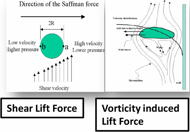
Figure 8: Saffman-Mei model and the Moraga model calculate the lift coefficient by combining two different physical effects.

Legendre-Magnaudet Model

The Legendre-Magnaudet model is a special formulation that looks at the inside of the bubble. When a bubble moves, the gas inside it also circulates. This model includes the effect of that internal gas circulation by combining the bubble Reynolds number with the dimensionless shear rate of the liquid. You should use the Legendre-Magnaudet model when you only have small, perfect spherical bubbles that do not change shape.

Figure 9: Gas circulation inside the bubble as it moves

Tomiyama Lift Model

When bubbles grow very large, they become flat or look like a cap. Because of this new shape, the lift force actually changes direction. Instead of pushing the bubbles to the wall, the fluid pushes large cap bubbles toward the center of the pipe. The Tomiyama model uses a modified Eotvos number to calculate this exact bubble deformation and mathematically accounts for this sign change. You should always use the Tomiyama lift model when you have all different shapes and sizes of bubbles, because it correctly pushes small bubbles to the wall and large bubbles to the center.

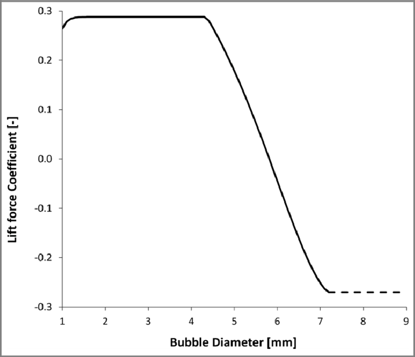
Figure 10: Dependence of lift force coefficient on bubble diameter

Figure 11: Diagram showing the lift force pushing small spherical bubbles to the wall and large ellipsoidal bubbles to the center of the pipe.

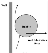
Wall Lubrication Force

When bubbles move near a solid wall, they naturally experience a force that pushes them away from the surface. This physical push is called the wall lubrication force. In real life, experiments show that there is a zero-gas volume fraction right next to vertical walls because this force prevents the bubbles from touching the solid boundaries.

In the Eulerian multiphase model, the general governing equation for the wall lubrication force () is defined as the negative wall lubrication coefficient () multiplied by the continuous liquid density, the gas volume fraction, the square of the slip velocity parallel to the wall, and the wall normal vector. To solve this governing equation correctly in your gas-liquid flow CFD project, ANSYS Fluent offers several specific models to calculate the exact coefficient.

$F_{WL} = C_{WL} \alpha_p \rho_q | \vec{v}_p - \vec{v}_q |_{||} \vec{n}_w$

Figure 12: Lift coefficient models available in Forces tab of Eulerian multiphase model in ANSYS Fluent

Antal et al. model

The Antal et al. model is the most basic choice for wall lubrication. The governing equation for the Antal coefficient mathematically compares the bubble diameter (Dh) to the physical distance to the wall (Yw) using the formula

$C_{WL} = \max (0, \frac{-0.01}{d_b} + \frac{0.05}{y_w})$

You must use the Antal model when your simulation only has very small bubbles. Because this mathematical formula is only active in a very thin region close to the wall, you must create a very fine mesh near your boundaries, or the software will not calculate the force correctly.

Tomiyama Model

The Tomiyama model is a special modification of the Antal model made specifically for pipe flows. The governing equation for the Tomiyama coefficient uses the total pipe diameter (D) and the distance to the wall (Yw) in the formula

$C_{WL} = C_w \frac{d_b}{2} (\frac{1}{y_w^2} - \frac{1}{(D-y_w)^2})$

where the value Cw depends heavily on the Eotvos number to account for bubble deformation. You must use the Tomiyama model when you have viscous fluids and all different sizes and shapes of bubbles flowing inside a pipe. It is highly recommended for standard air-water systems because it perfectly calculates how bubble shape changes the wall force.

Frank model

The Frank model is a very smart upgrade to the Tomiyama model. The Tomiyama model needs the exact pipe diameter, which is a big problem if you are simulating a complex tank instead of a simple pipe. The governing equation for the Frank model removes the pipe diameter completely and instead uses a mathematical cut-off distance based on the bubble diameter to make the formula geometry independent. You must always use the Frank model when you have complex geometries that are not simple pipes, but you still need to accurately model viscous fluids and all variable bubble shapes.

Hosokawa model

The Hosokawa model is another excellent choice that looks at the physical fluid properties using the Morton number. The governing equation for the Hosokawa coefficient directly compares the Eotvos number () and the bubble Reynolds number (Re) using the mathematical formula

$C_{WL} = \max (\frac{7}{Re^{1.9}}, 0.0217Eo)$

You must use the Hosokawa model when you want the software to accurately include the physical effects of the relative Reynolds number for all bubble sizes and shapes in low-velocity flows.

Virtual Mass Force

When a bubble suddenly speeds up or slows down in a liquid, it must also push the heavy fluid around it. This creates an extra resistance. We call this the virtual mass force. Imagine dipping your palms into water and bringing them together very slowly; it requires little effort. Now, try to clap your hands quickly underwater. The high acceleration requires a huge effort because you are moving the mass of the water. This is exactly how the virtual mass force works.

In the software, the governing equation for the virtual mass force depends on the relative acceleration between the phases. The mathematical governing equation is

$F_{vm} = C_{vm} \alpha_p \rho_q (\frac{D_q v_q}{Dt} - \frac{D_p v_p}{Dt})$

In this formula, Cvm is the virtual mass coefficient, Alpha(p) is the secondary phase volume fraction, rho-q is the liquid density, and the remaining terms represent the phase accelerations. For most bubbly flows, the virtual mass coefficient Cvm is simply set to a constant value of .

You must use the virtual mass force when the continuous primary phase density is much larger than the dispersed secondary phase density, like in air-water bubbly flows. It is extremely important to activate this force for transient flows where bubbles oscillate or vibrate. You must also use the virtual mass force in strongly accelerating flows, for example, when a bubbly liquid travels very fast through a narrow pipe constriction. You do not need to use this force for solid granular flows because the density difference is small.

Turbulent Dispersion Force

In highly turbulent flows, chaotic fluid eddies hit the bubbles and mix them into the continuous phase. This mixing process is called the turbulent dispersion force. The main physical effect of this force is to push bubbles away from crowded areas to make the gas distribution more uniform.

Figure 13: Diagram showing the turbulent dispersion force pushing bubbles from high concentration areas to create a uniform flow.

In ANSYS Fluent, the basic governing equation for this force uses a gradient transport method. The general governing equation is defined as the turbulent dispersion coefficient (Ctd) multiplied by the liquid density, the turbulent kinetic energy, and the mathematical gradient of the gas volume fraction. To calculate this exact force, you can choose from several specific mathematical models.

Figure 14: ANSYS Fluent Turbulent dispersion force models

Lopez de Bertodano model

The Lopez de Bertodano model is a very popular choice for calculating the dispersion force. Its governing equation directly uses the turbulent kinetic energy (Kq) of the continuous phase to find the force. You must use the Lopez de Bertodano model with a coefficient between 0.1 and 0.5 when your tank has medium-sized ellipsoidal bubbles. However, if your simulation only has very small spherical bubbles, you must use a much higher coefficient up to 500.

Burns et al. model

The Burns et al. model is a more advanced option that uses a strict mathematical derivation based on Favre averaging. Its governing equation calculates the dispersion force using the specific turbulent diffusivities of the phases instead of simple kinetic energy. You must use the Burns et al. model for standard bubbly flows where the particle relaxation time is very short compared to the fluid turbulence time.

Simonin model

The Simonin model is another available option, but it uses the exact same mathematical formulation and rules as the Burns model.

Diffusion in VOF model

Finally, instead of adding a direct momentum force, you can select the Diffusion in VOF model to physically add a turbulent diffusion term directly into the mass continuity equation to completely homogenize the flow.

Summary & Recommendations

Simulating gas-liquid flows in the Eulerian multiphase model requires a very careful selection of interphase forces. You must always start your gas-liquid flow CFD project by choosing the correct drag model based on your exact bubble size and flow regime. If your liquid rotates or changes speed, you must add the lift force to push bubbles in the correct radial direction. If your bubbles move near solid boundaries, you must turn on the wall lubrication force to prevent them from touching the vertical walls. Finally, you must add the virtual mass force for rapidly accelerating bubbles and the turbulent dispersion force to mix the bubbles smoothly in turbulent flows. Always evaluate your exact physical problem before turning on these advanced non-drag forces, because adding unnecessary forces will make your mathematical solver very slow and unstable.

Frequently Asked Questions (FAQ)

What is the difference between drag and non-drag forces in ANSYS Fluent? The drag force acts exactly in the opposite direction of the bubble movement to create a direct hydrodynamic resistance. Non-drag forces act in completely different directions or only under very special conditions. For example, the lift force pushes bubbles sideways across the pipe, the wall lubrication force pushes them away from solid metal boundaries, and the virtual mass force only acts when the bubbles suddenly change their speed.
When must I activate the virtual mass force in my simulation? You must always activate the virtual mass force when your continuous primary fluid is much heavier than your dispersed secondary bubbles. If you are simulating light air bubbles accelerating inside heavy liquid water, the virtual mass force is strictly required to calculate the extra effort needed to move the surrounding heavy fluid. You do not need to use this force for heavy solid particles falling in light air.
Why do the large bubbles in my simulation collect incorrectly at the pipe wall? Small spherical bubbles naturally move toward the wall because of the classical aerodynamic lift force. However, if your bubbles are large and they still collect at the wall, you are using the wrong mathematical lift model. You must change your settings and select the Tomiyama lift model. The governing equation for the Tomiyama model uses a modified Eotvos number to mathematically change the sign of the lift coefficient, which correctly pushes large cap bubbles back toward the center of the pipe.
How does the software know when a bubble changes from a sphere to a large cap shape? ANSYS Fluent uses an automatic flow regime detection tool inside the Grace and Tomiyama drag models. The software mathematical solver calculates the drag coefficient for viscous, distorted, and cap shapes all at the exact same time. The governing equation automatically selects the correct bubble shape by mathematically finding the minimum or maximum drag value between these three different flow regime curves.
Can I use the Eulerian multiphase model for solid granular flows instead of gas bubbles? Yes, you can use this exact model for solid particles, but you must enable the Eulerian Granular model settings. For granular flows, the physical collisions between the hard particles are the most dominant forces. Therefore, you do not need to use fluid forces like wall lubrication or virtual mass. Instead, the governing equations will calculate the solid pressure and granular temperature to model the kinetic particle collisions accurately.

Interphase Forces in Eulerian Model: Drag and Non-Drag Forces

Overview of Interphase Forces