

![The 3D Velocity vectors showing the fluid accelerating through the bottom cone to a maximum of 8.96 [m s^-1].](https://cfdland.com/wp-content/uploads/2026/06/vec.webp)
![The 3D Temperature streamlines showing hot and cold flows twisting together from 300 to 400 [K].](https://cfdland.com/wp-content/uploads/2026/06/tsrre.webp)
![The Local Sensitivity chart proving the hot inlet Velocity dominates the chamber Pressure Drop by exactly 86 [%].](https://cfdland.com/wp-content/uploads/2026/06/sensitivity.webp)
![The 3D Response Surface showing the Temperature Spread reaching a high red peak near 0.045 [K] when fluids move too fast.](https://cfdland.com/wp-content/uploads/2026/06/RSM-temp.webp)
![The 3D Response Surface proving Pressure Drop increases smoothly to exactly 210 [Pa] as the inlet momentum rises.](https://cfdland.com/wp-content/uploads/2026/06/RSM-p.webp)
Thermal mixing chambers are very important pipes in factories. They take two different fluids and mix them into one uniform output. A good chamber must have perfect fluid balance. If the fluid moves too fast, it crashes hard into the walls. This crash creates a high pressure drop, which forces the factory pumps to waste a lot of energy. If the fluid moves too slow, the hot and cold parts do not mix. This creates dangerous hot spots that can destroy the pipe.
Engineers must find the exact perfect speed for the fluid. Testing every speed by hand takes too much time. Today, we use smart computer math to do this automatically. If you want to master these advanced math tools, studying our professional heat transfer CFD simulation projects is the best step. In this tutorial, we combine ANSYS Fluent, CFD-Post, and DOE–RSM optimization techniques to identify the optimal operating conditions that minimize temperature non-uniformity and pressure losses inside the mixing chamber.
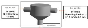
Figure 1: Schematic outline of the mixing chamber and Boundary conditions
Simulation Process: Essential Optimization Models
To build this simulation correctly, we must use the exact scientific models and boundary conditions without any extra filler. We define a cold air inlet at exactly 300K with a velocity range of 0.5 to 1.5m/s . We define a hot air inlet at exactly 400K with a velocity range of 1.5 to 3.5 [m/s].
To optimize this, we use the Design of Experiments (DOE) tool combined with the Response Surface Methodology (RSM). We apply the Optimal Space-Filling design method. This specific mathematical model automatically tests exactly 20 different design points across the entire physical range. We set two strict physics goals: minimize the Temperature Spread (Standard Deviation) and minimize the Pressure Drop. Finally, we use the Screening optimization method. This model scans the math results to find the absolute best combination of fluid speeds.
Post-processing: Physics of Fluid Momentum and Thermal Blending
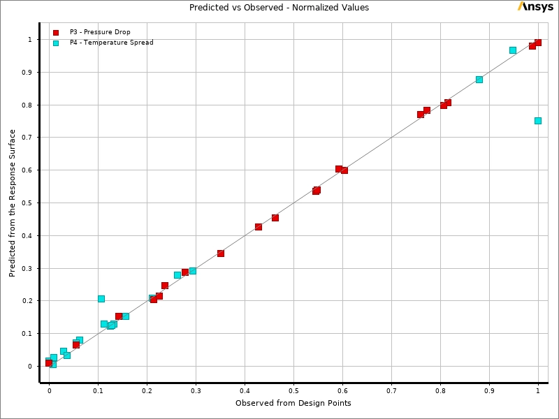
We will now analyze the rich visual data produced by the mathematical optimization software. We must study how the fluid behaves when we change the speeds. We begin by looking at the Predicted versus Observed chart. This graph proves if the computer learned the physics correctly. The red squares represent the Pressure Drop. They sit almost perfectly on the straight diagonal line. This proves the mathematical model can predict flow friction changes with very high accuracy. The cyan squares represent the Temperature Spread. They also follow the main line closely. Because both data sets align tightly, we know the response surface model is highly reliable. We can trust this math to find the best fluid speeds without running hundreds of extra simulations.
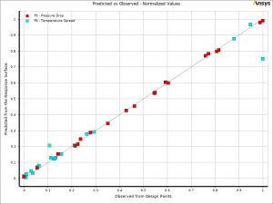
Figure 2: The Predicted versus Observed chart proving the mathematical surface accurately predicts the Pressure Drop and Temperature Spread.
Next, we study the three-dimensional response surface charts. These mathematical shapes show us exactly how the input speeds change the physical results. We look first at the Temperature Spread surface. The color map shows a bright red mountain peak. This high peak happens when the cold speed is high near 1.5 [m s^-1] and the hot speed is high near 3.0 [m s^-1]. This red zone is the worst possible operating region because the Temperature Spread reaches a maximum near exactly 0.045 [K]. The fluids move too fast and fail to mix. To fix this, we look for the deep blue valley on the surface map. This optimal blue zone appears when the cold speed is low near 0.5 [m s^-1]. Reducing the cold energy gives the hot fluid enough physical time to blend completely inside the cylinder.
We then examine the Pressure Drop surface chart. This geometric shape is very smooth and slopes upward like a ramp. The colors change from dark blue at the bottom to bright red at the top. The maximum pressure resistance reaches exactly 210 [Pa]. This high resistance happens when both pipes push fluid at their maximum speed limits. The minimum resistance is found in the deep blue corner, resting near exactly 90 [Pa]. This physical shape proves that high flow momentum directly causes high fluid friction against the solid metal walls.
![The 3D Response Surface showing the Temperature Spread reaching a high red peak near 0.045 [K] when fluids move too fast.](https://cfdland.com/wp-content/uploads/2026/06/RSM-temp-300x225.webp)
Figure 3: The 3D Response Surface showing the Temperature Spread reaching a high red peak near 0.045 [K] when fluids move too fast.
![The 3D Response Surface proving Pressure Drop increases smoothly to exactly 210 [Pa] as the inlet momentum rises.](https://cfdland.com/wp-content/uploads/2026/06/RSM-p-300x225.webp)
Figure 4: The 3D Response Surface proving Pressure Drop increases smoothly to exactly 210 [Pa] as the inlet momentum rises.
To understand exactly which pipe controls these physical results, we look at the Local Sensitivity chart. The blue bar represents the hot fluid speed. The red bar represents the cold fluid speed. For the Pressure Drop, the hot pipe is the absolute most important part. It controls exactly 86 [%] of the physical pressure change. The cold pipe only controls exactly 32 [%]. However, for the Temperature Spread, the control is shared equally. The hot pipe drives exactly 42 [%], while the cold pipe drives exactly 25 [%]. This proves that achieving a perfectly mixed temperature requires careful mathematical control of both fluid streams together.
![The Local Sensitivity chart proving the hot inlet Velocity dominates the chamber Pressure Drop by exactly 86 [%].](https://cfdland.com/wp-content/uploads/2026/06/sensitivity-300x225.webp)
Figure 5: The Local Sensitivity chart proving the hot inlet Velocity dominates the chamber Pressure Drop by exactly 86 [%].
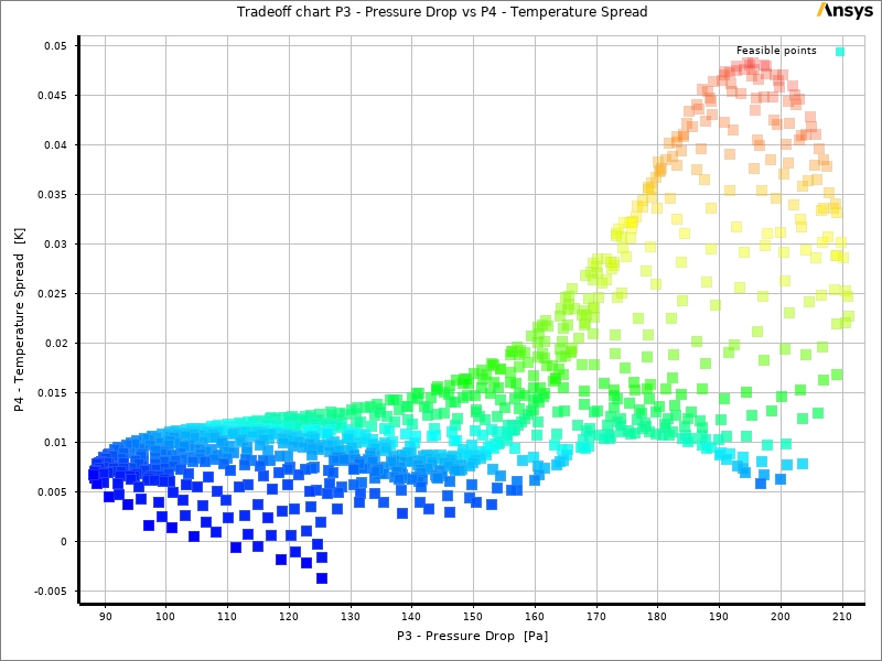
We use the Pareto Tradeoff chart to find the final physical solution. This graph plots every possible operating condition. We want low friction and low thermal spread. Therefore, the perfect design must sit in the bottom left corner. The software highlights a dense cluster of blue squares in this exact region. This is the optimal design zone. From this optimal blue zone, the software automatically selects three perfect candidates.

Figure 6: The Pareto Tradeoff chart revealing the optimal blue cluster where both thermal spread and pressure loss are minimized.
The table below shows the three best candidate points chosen by the mathematical screening tool.
| Candidate | Cold Velocity [m s^-1] | Hot Velocity [m s^-1] | Predicted Pressure Drop [Pa] | Predicted Temp Spread [K] |
| Point 1 | 1.0125 | 1.5030 | 97.212 | 0.0016420 |
| Point 2 | 1.2685 | 1.5069 | 111.440 | -0.0005860 |
| Point 3 | 1.5000 | 1.5000 | 125.350 | -0.0037105 |
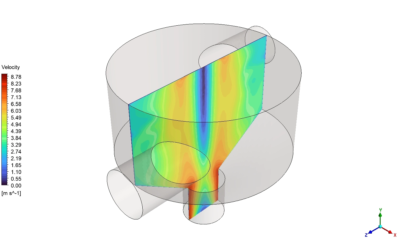
We select Candidate 2 as the absolute best design. The software validates this design with a full fluid flow simulation. We look at the final Velocity vectors. The legend shows the speed ranges from exactly 0.00 to 8.96 [m s^-1]. The hot and cold jets enter the main chamber and crash into each other violently. This crash creates a strong spinning fluid vortex in the upper cylinder. The fluid then accelerates sharply down the exit cone, turning solid red at the peak speed of exactly 8.96 [m s^-1].
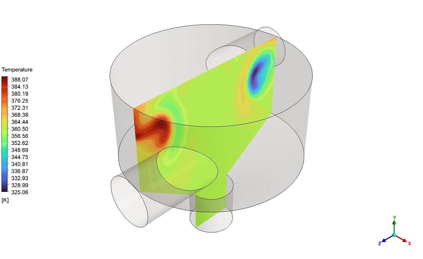
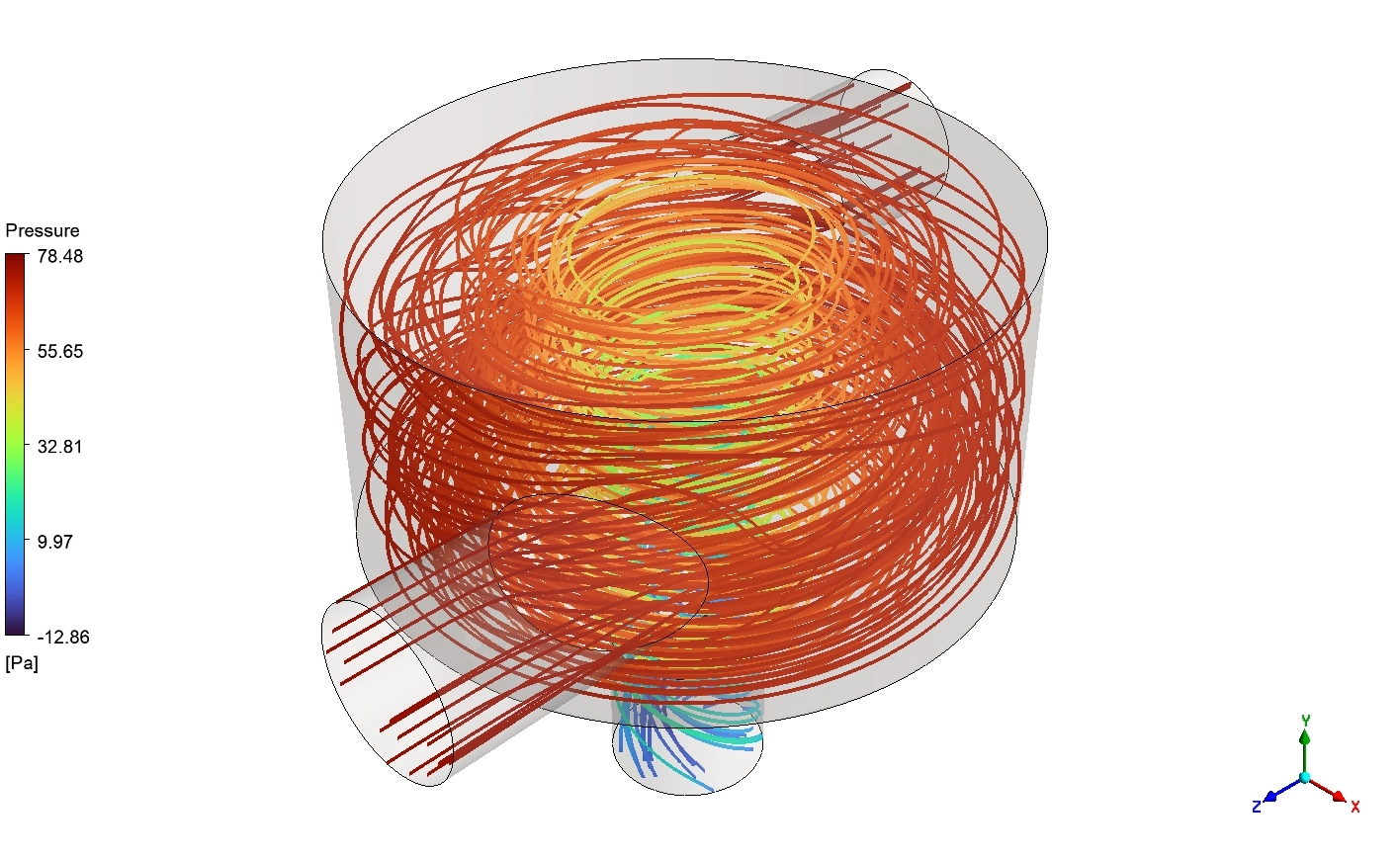
Finally, we analyze the 3D fluid streamlines colored by Temperature. The legend goes from exactly 300 to 400 [K]. The spinning vortex forces the extreme hot red lines and cold blue lines to twist tightly together. Because the inlet speeds are perfectly balanced by the software, the fluids mix before reaching the bottom hole. The final validated design physically achieves an excellent low pressure drop of exactly 104.166 [Pa] and a tiny temperature spread of exactly 0.00555837 [K]. The mathematical optimization is a complete success.
![The 3D Velocity vectors showing the fluid accelerating through the bottom cone to a maximum of 8.96 [m s^-1].](https://cfdland.com/wp-content/uploads/2026/06/vec-300x184.webp)
Figure 7: The 3D Velocity vectors showing the fluid accelerating through the bottom cone to a maximum of 8.96 [m s^-1].
![The 3D Temperature streamlines showing hot and cold flows twisting together from 300 to 400 [K].](https://cfdland.com/wp-content/uploads/2026/06/tsrre-300x184.webp)
Figure 8: The 3D Temperature streamlines showing hot and cold flows twisting together from 300 to 400 [K].
Frequently Asked Questions (FAQ)
- Why do we use Response Surface Methodology (RSM)?
- Testing every single fluid speed takes too much computer time. The RSM math tool takes just 20 tests and builds a complete, highly accurate 3D map of the physics. This saves massive time while finding the absolute best design.
- Why does a high velocity cause a massive pressure drop?
- Fluid behaves like a solid force when it moves fast. If you push the fluid too hard into the pipe, it crashes into the metal walls. This crash turns into mechanical friction. We measure this heavy friction as high Pressure Drop.
- How does the shape of the chamber help the temperature mix?
- The two fluids enter from opposite sides into a wide cylinder. When they crash in the middle, they have nowhere to go but spin. This geometric shape forces a massive tornado. This spinning motion gives the hot and cold molecules the exact physical time they need to share their heat.


Reviews
There are no reviews yet.