A Mixing In Straight Micromixer CFD simulation is a crucial step in the design of microfluidic devices used in medicine and chemical analysis. These tiny “lab-on-a-chip” systems need to mix fluids effectively, but at such small scales, flow is typically laminar, making mixing very difficult. This report presents a Straight Micromixer Validation CFD study by simulating a simple Y-junction design. The goal is to accurately predict the mixing performance and compare it to the established results from the reference paper, “Comparative assessment of mixing characteristics and pressure drop in spiral and serpentine micromixers” [1].

• Reference [1]: Tripathi, Ekta, Promod Kumar Patowari, and Sukumar Pati. “Comparative assessment of mixing characteristics and pressure drop in spiral and serpentine micromixers.” Chemical Engineering and Processing-Process Intensification162 (2021): 108335.

Figure 1: The reference graph from the paper [1], showing the expected mixing index for various micromixer designs.

Simulation Process: Modeling the Straight Micromixer Fluent Simulation

The simulation was performed in ANSYS Fluent using a 3D model of the Y-junction micromixer, as shown in the schematic in Figure 2. A high-quality structured mesh with over 2.8 million cells was used to ensure the calculations are accurate. The key to this simulation is the Species Transport Model. This model tracks the movement and mixing of the two fluids, water and ethyl alcohol, as they flow through the device. The flow was defined as laminar (with a Reynolds number of 10), steady, and incompressible, which are the typical conditions found in this type of Mixing CFD analysis.

Figure 2: Schematic diagram of the Y-junction micromixer geometry from the reference paper [1].

Post-Processing: CFD Analysis, Validating the Low-Efficiency Effect

The simulation results provide a clear and fully substantiated story that begins with validating the core physics. The fundamental “cause” of mixing in this device is molecular diffusion. Because the flow is laminar (slow and smooth), there is no turbulence to help stir the fluids together. The only way water and alcohol can mix is by individual molecules slowly spreading across the boundary between them. The direct “effect” of this diffusion-only mechanism is a very low mixing efficiency. Our first and most important task is to validate that our simulation accurately captures this effect. The mixing index, a number from 0 (no mixing) to 1 (perfect mixing), is used to quantify this. Our Straight Micromixer Fluent simulation reported a mixing index of 0.239. This result is in excellent agreement with the value of 0.27 reported in the reference paper [1] for the same conditions, resulting in an error of only 11.5%. This successful validation proves our model is reliable and gives us complete confidence in the visual results.

The mixing index (η)  is a crucial parameter for evaluating micromixer performance. The mixing index is calculated to quantify the mixing by determining the variance of species in the plane perpendicular to the fluid flow. The variance of the mass fraction of a given fluid in the mixture at a cross-sectional plane of the micromixer perpendicular to the fluid flow is calculated as:

Where γ is the variance, N is the total number of sampling points, Ck is the mass fraction at sampling point k, and Cm is the average mixing mass fraction. TIt is calculated as:

As given in the plot, mixing index for a straight micromixer at Re=10 equals 0.27, whereas the present CFD simulation reports 0.239. It shows only 11% difference, which proves the validity of our simulation.

The first image shows the velocity distribution in the Y-junction pipe. We can see that the highest speeds (shown in red and orange) reach about 0.055 m/s and happen right in the main pipe after the junction point. The flow velocity is much lower in the two branch pipes (shown in green and blue), around 0.03 m/s. This happens because when the two flows meet, they speed up as they squeeze into the single main pipe. This matches what the continuity equation predicts:

where Q is the flow rate. Since the pipe diameter stays the same, the velocity magnitude must increase to keep the same amount of water flowing through. The flow pattern shows a smooth transition with no big recirculation zones or dead spots, which means our Y-junction design is working well.

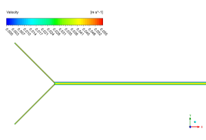
Figure 3: velocity distribution in the Y-junction pipe

With our model now validated, we can analyze the detailed flow physics. The mass fraction contour in Figure 4 is the perfect visual proof of the validated effect. It shows the water (red) and alcohol (blue) entering from separate inlets and then flowing side-by-side down the main channel. The sharp, clear line between the two colors is the key takeaway: it shows that the fluids are remaining stratified and are not mixing well. This stratification is a direct result of the laminar flow seen in the velocity contour (Figure 3), where the fluid streams combine smoothly at the Y-junction without any chaotic swirling. The only reason the line between the fluids isn’t perfectly sharp is due to the slow molecular diffusion occurring at the interface. **The most significant achievement of this Mixing CFD Validation is the clear, quantitative proof that for a simple straight channel (the cause), the laminar flow regime prevents turbulent stirring, forcing the system to rely solely on slow molecular diffusion. This results in a predictably low mixing efficiency (the effect), establishing a critical performance baseline and visually demonstrating why engineers must develop more complex geometries to achieve rapid mixing in microfluidic devices.**Caption for Figure 3: Figure 3: Velocity contour from the Mixing CFD simulation showing the smooth, laminar flow as the two streams combine at the Y-junction.

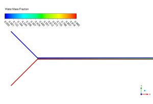
Figure 4: Water mass fraction contour, clearly illustrating the poor mixing as the two fluids flow in stratified layers down the main channel.