
Modeling turbulence in multiphase flows is a very complex and difficult task. In a simple single-phase flow, the fluid mixes naturally because of standard velocity changes. We call this basic mixing shear-induced turbulence. However, when you add a secondary phase like gas bubbles or solid particles into the fluid, the physical mixing process changes completely. To get accurate results in your CFD project, you must mathematically calculate how the two phases change the turbulence of each other at the exact same time. If you want to learn exactly how to set up these specific boundaries and models in the software, we highly recommend practicing with our step-by-step Multiphase tutorials.
When bubbles move inside a liquid, their physical presence distorts the fluid streamlines. This distortion creates a new type of mixing called bubble-induced turbulence or turbulence modulation. The size and concentration of your bubbles will directly decide how the continuous fluid behaves. For example, large bubbles create strong wakes behind them as they move. These large wakes will greatly increase the total turbulence levels in the continuous liquid. On the other hand, if you have a very large number of extremely small bubbles, they will actually absorb the energy and decrease the turbulence in the continuous liquid.
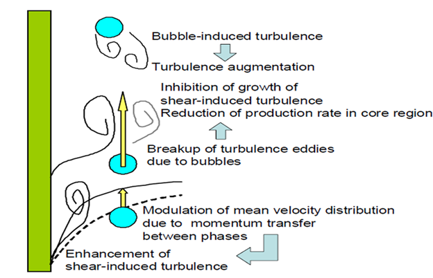
Figure 1: Turbulence in multiphase flows is highly complex due to the physical interaction between fluid shear eddies and bubble-induced wakes.
In a realistic Eulerian multiphase simulation, the natural shear-induced turbulence and the new bubble-induced turbulence do not act alone. There is a very strong and direct interaction between them. The chaotic fluid eddies continuously hit the bubbles, while the moving bubbles continuously break and change the fluid eddies. Because of this highly complex two-way interaction between the fluid shear and the moving bubbles, you must carefully select specific multiphase turbulence models in ANSYS Fluent to accurately simulate your project.
Turbulence Model Options in Fluent (k-ε and k-ω)
When you simulate a gas-liquid flow CFD project in ANSYS Fluent, the software gives you three different ways to calculate the chaotic flow using the standard k-epsilon or k-omega models in the Eulerian multiphase model. The first and most basic option is the mixture turbulence model. This is the automatic default setting in the software. It works by mathematically calculating a single set of shared mixture properties and mixture velocities for the entire domain. You must use the mixture turbulence model when your flow separates into distinct stratified layers or when the physical density ratio between your two phases is very close to 1. Because it only solves one basic governing equation for the turbulent kinetic energy and one for the dissipation rate, it is mathematically very fast and stable.
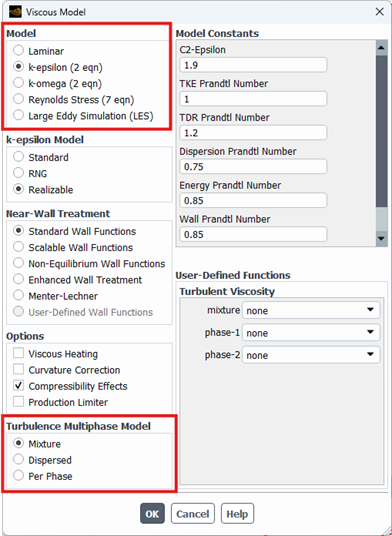
Figure 2: Eulerian Turbulence models provided in ANSYS Fluent
The second option is the dispersed turbulence model. In this mathematical method, the chaotic turbulence of the primary continuous phase directly influences and controls the random motion of the secondary phase. The governing equation for the primary phase turbulent kinetic energy adds a special mathematical source term to account for the physical presence of the bubbles. This governing equation is written as:

In this formula,  is the volume fraction,
  is the density,
  is the turbulent viscosity,
  is the turbulence production, and
  is the extra mathematical source term from the dispersed bubbles. You must use the dispersed turbulence model when you have one clear primary continuous liquid and a very dilute or small concentration of secondary dispersed bubbles.
The third and most advanced option is the per-phase turbulence model. This mathematical model is completely different from the others because it solves separate and individual turbulence governing equations for each separate phase in the tank. You must use the per-phase turbulence model when the physical turbulence transfer among the different phases plays a very dominant and highly important role in your project. Because the mathematical solver must calculate completely separate turbulent kinetic energy and dissipation equations for every single fluid in your domain, this model requires a lot of computer memory but gives highly accurate results for complex mixing problems.
Reynolds Stress Models (RSM) for Multiphase
Sometimes, the standard k-epsilon or k-omega models are not mathematically strong enough to capture highly complex fluid motions. In simple pipes, fluid turbulence is generally the same in all directions. However, in complex rotating flows, the chaotic eddies stretch and become completely different in every physical direction. To capture this complex physics, you must use the Reynolds Stress Model (RSM). Instead of using a simple turbulent viscosity assumption, the RSM solves separate governing equations for the exact turbulent stress tensor in every single direction.
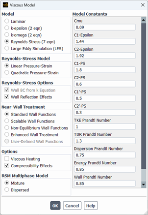
Figure 3: RSM turbulence model for tracking eddies in Eulerian multiphase flow
For multiphase flows, ANSYS Fluent provides two specific RSM options. You can choose either the mixture RSM or the dispersed RSM. The mixture RSM calculates the directional stresses for the combined fluid, while the dispersed RSM calculates how the primary fluid stresses affect the secondary phase. You must use the Reynolds Stress Model when your project includes highly swirling flows, strong separation cyclones, or severe rotating secondary flows. You must be very careful when using the RSM because solving these advanced directional governing equations requires huge computational power and can easily make your numerical solver unstable.
Figure 4: A dense swirling cyclone perfectly demonstrates a complex flow where the advanced Dispersed Reynolds Stress Model (RSM) is strictly required.
Turbulence Interaction Models
When bubbles move through a liquid, their wakes create new chaotic eddies. In the software, you must select a specific turbulence interaction model to calculate this exact bubble-induced turbulence. The first available option is the Sato model. The Sato model does not add any complex mathematical source terms to your main kinetic energy equations. Instead, it simply adds a new particle-induced turbulent viscosity to the normal fluid shear viscosity. Its exact governing equation is written as:

You should use the Sato model when you have a very low concentration of bubbles and you want a fast, mathematically stable simulation.
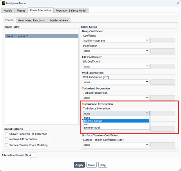
Figure 5: The Turbulence Interaction tab inside the Phase Interaction panel allows you to choose exactly how bubbles create extra turbulence.
The second option is the Simonin model. This mathematical model is much more advanced because it directly adds new physical source terms to both the turbulent kinetic energy and the dissipation rate equations. Its governing equation calculates the kinetic energy source term using the exact energy transfer time between the eddies and the particles, written as:

You must use the Simonin model only when you activate the dispersed or per-phase turbulence options to strictly calculate the complex energy transfer between your phases.
The final option is the Troshko-Hassan model. This model serves as an excellent alternative to the Simonin model. Its governing equation calculates the mathematical source term by directly using the relative velocity difference between the phases, written as:

We highly recommend using the Troshko-Hassan model when you need extremely accurate turbulence results very close to the gas injection points at the bottom of your bubble column.
Conclusion
Simulating turbulent multiphase flows requires much more than standard single-phase equations. You must carefully define how the continuous liquid and the secondary bubbles mix together to get highly accurate results in your CFD project. We explored the deep physical differences between normal shear eddies and complex bubble-induced wakes. By selecting the correct mathematical formulation in the software, such as the fast mixture model or the highly detailed per-phase model, you perfectly capture the chaotic movement of your fluids. We also learned how adding specific interaction equations, like the Sato or Troshko-Hassan models, directly calculates the extra energy created by the rising bubbles. Choosing the correct multiphase turbulence settings is absolutely critical because it directly controls the flow behavior, the mixing quality, and the final scientific accuracy of your entire industrial simulation. If you want to deeply master these advanced software setups and apply them directly to your own engineering projects, we highly invite you to explore our comprehensive Multiphase Tutorials. These practical step-by-step guides will help you simulate any complex fluid interaction with complete confidence.