Eulerian Granular Model – Modeling Particulate Flows in ANSYS Fluent

Particulate flows happen everywhere in the real world and across many major heavy industries. Engineers constantly use CFD to simulate solid particles moving inside a fluid for oil and gas refineries, chemical processing plants, pharmaceutical factories, food processing facilities, and deep mining projects. In these complex gas-solid or liquid-solid flows, the small solid particles interact very strongly with the surrounding continuous fluid. To mathematically calculate these highly complex physical interactions with true accuracy, you must use the advanced Eulerian Granular Model in your simulation software.

When you start a new particulate flow project, you must first look at your exact particle concentration to understand the physical coupling. If your tank has a very low number of particles with large empty spaces between them, we call this a dilute flow. In dilute flows, you usually have basic one-way or two-way coupling, which simply means the main fluid pushes the particles, and sometimes the moving particles push the fluid back. However, if your tank contains a massive number of particles packed closely together, we call this a dense flow. In highly dense flows, you must strictly calculate four-way coupling because the fluid pushes the particles, the particles push the fluid back, and the particles constantly crash into each other at the exact same time.

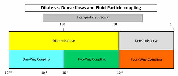
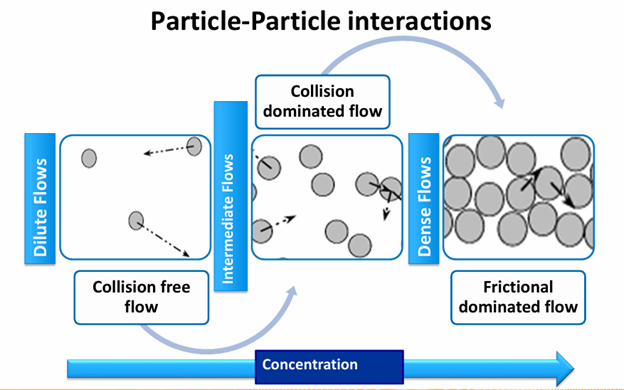
Figure 1: A physical regime map showing how increasing the particle volume fraction completely changes the flow from a simple collision-free state to a highly dense friction-dominated state.

Depending on the total volume fraction of your solids, the mathematical solver will see three completely different physical particle-particle interactions. In very dilute concentrations, you have a simple collision-free flow because the particles have too much empty space and rarely touch each other. As the particle concentration increases to an intermediate level, the flow changes into a collision-dominated state where fast particles continuously hit and bounce off each other. Finally, when the solid particles are packed very tightly together at the maximum physical limit, the flow becomes friction-dominated because the particles do not have any empty space to bounce, so they just constantly rub against each other. If you want to learn exactly how to simulate all of these complex particle regimes in the software, we highly recommend practicing with our step-by-step Multiphase CFD simulation tutorials.

 

Granular Flow Regimes

When millions of solid particles move together inside an industrial tank, their physical behavior completely changes based on their speed and how closely they are packed. To accurately simulate these particles, scientists divide this complex movement into three completely different physical categories.

Here are the three distinct granular flow regimes:

• 1. The Quasi-Static Regime (Very Slow Flow): This physical condition happens when the particles are packed very tightly together and move extremely slowly, exactly like heavy dirt moving in soil mechanics. Because the particles do not have space to bounce, they just constantly rub against each other. In this slow state, the mathematical solid stress is completely independent of the flow speed (the strain rate, ). The exact mathematical equation is written as

• 2. The Intermediate Regime (Medium Flow): This is the middle transition state. The particles start to move a little faster and have a little bit more empty space between them. Because the flow is faster, the mathematical solid stress starts to depend on the physical strain rate. The governing equation relates the stress to the strain rate using a fractional power, written exactly as (where the value of is strictly between zero and two).
• 3. The Inertial Regime (Rapid Flow): This happens in very fast and highly rapid flows where the particles fly freely and violently crash into each other. Because the particles hit each other with very high kinetic energy, the physical stress depends heavily on the square of the flow speed. The mathematical equation for this rapid regime is written as

You must clearly understand these three physical categories because the software uses the advanced Kinetic Theory of Granular Flow (KTGF) to solve the rapid inertial regime, but you must strictly activate different frictional stress equations to correctly solve the slow quasi-static regime.

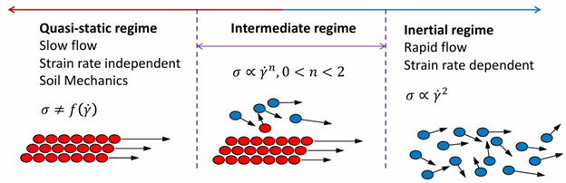
Figure 2: The granular regime map shows exactly how the physical stresses change from slow friction-dominated movements to rapid collision-dominated flows.

Why We Need the Granular Model

If you try to simulate a large number of particles using the basic Eulerian-Eulerian model, the software will calculate completely wrong physical results. The basic model only sees the particles as a simple fluid and allows them to pack together infinitely without any natural resistance. To stop this physical error, you must use the advanced Eulerian Granular Model. This model adds special mathematical equations for solids pressure and granular viscosity, which physically force the particles to bounce off each other and correctly resist heavy packing.

To completely prove why this advanced model is absolutely necessary, we can look at the main graphical contours from our professional Multiphase CFD simulation tutorials. Here are three practical examples showing the power of the granular model:

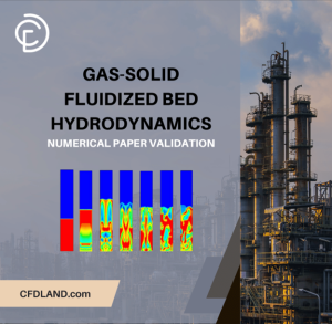
• Gas-Solid Fluidized Bed Hydrodynamics CFD Simulation: In this numerical paper validation, the granular equations perfectly calculate the exact Voidage Profile. This crucial contour represents the empty space (air) in the mixture and accurately shows three distinct zones: a dense lower zone, a transitional region, and a dilute upper region. Because the model calculates the particle collisions correctly, you can clearly visualize the Solid-phase volume fraction and the complex Bubble behavior showing the formation, expansion, and coalescence of bubbles with errors not exceeding 10%. We even extract the Residence Time Distribution (RTD) to validate the highly accurate dynamic behavior against experimental data.
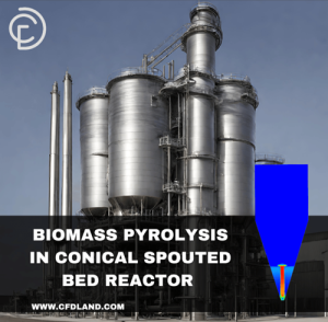
• Biomass Pyrolysis in Conical Spouted Bed Reactor CFD Simulation: In this complex reactor project, the granular physics are strictly required to create the correct flow shape. The main Solid particle volume fraction contour perfectly illustrates the characteristic “spouting” pattern, where a central high-speed jet drives the particle circulation. You can also clearly see the Velocity field driving the circulation and a very stable Temperature contour ranging from 372 K to over 729 K, proving the thermal mixing is highly accurate.
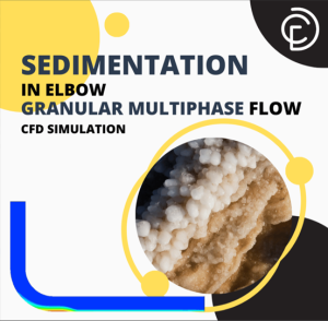
• Sedimentation in Elbow – Granular Multiphase Flow: In this ANSYS Fluent training, we simulate heavy particles moving inside a bent pipe. The primary contour is the volume fraction of the hydrate phase (R11). Because we use the physical granular equations, this contour visually represents exactly how the solid hydrates settle, rub against the walls, and heavily stratify at the bottom of the horizontal section due to gravity and changing viscosity gradients.

You must strictly enable the Eulerian Granular Model whenever your solid volume fraction is high enough for particles to touch or crash into each other, otherwise, your density and volume fraction contours will be completely physically wrong.

Kinetic Theory of Granular Flow (KTGF)

To mathematically calculate how millions of solid particles bounce and crash, the software uses the Kinetic Theory of Granular Flow (KTGF). This advanced framework is based exactly on the famous kinetic theory of gases, but it is modified specifically for solid spheres.

In a normal gas, tiny molecules bounce off each other perfectly without losing any speed. However, real solid particles have non-conservative physical interactions. This means every time two real solid spheres violently crash together, they permanently lose some of their bouncing energy because of inelastic collisions and physical friction. To accurately solve these complex physics, the KTGF strictly divides the particle movement into two completely different transport mechanisms:

• 1. Kinetic Transport (Free Flight): This physical mechanism happens when the solid particles fly completely freely through the empty fluid space. During this rapid free flight between the crashes, the moving particles carry their own physical kinetic energy.
• 2. Collisional Transport (The Crash): This physical mechanism happens at the exact moment when two or more particles violently hit each other. During this heavy crash, the particles physically transfer their momentum to each other and immediately lose energy.

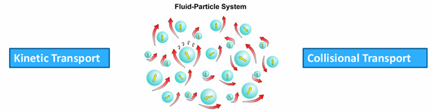
Figure 3: The Kinetic Theory of Granular Flow calculates both the free flight of particles (kinetic transport) and the violent crashes between them (collisional transport).

You must strictly use the KTGF equations to correctly calculate this physical energy loss and accurately capture the bouncing particle behavior in high-speed industrial processes.

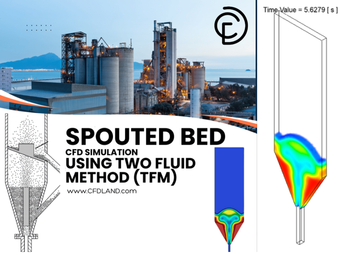
For a perfect practical example, you can look at our Spouted Bed CFD Simulation using Two Fluid Method (TFM) Training. In this specific complex reactor, the solid particles rapidly fly high up the central gas jet using pure kinetic transport, and then they heavily crash back down the side walls using pure collisional transport.

Granular Temperature

In the Eulerian Granular Model, the term “granular temperature” has absolutely nothing to do with real thermal heat. Instead, it is purely a mathematical concept used to measure the random bouncing energy of the solid particles. Just like hot gas molecules move much faster than cold ones, a high granular temperature simply means the solid particles are violently crashing into each other at very high speeds. Mathematically, it is defined as the average of the square of the fluctuating particle velocities, written simply as .

To accurately track this bouncing energy inside your tank, the software must solve a special transport equation. This complex equation carefully balances exactly how the kinetic energy is created, moved, and destroyed during the flow.

The particle energy naturally increases, called production, when the main fluid strongly pushes and shears the solids. Conversely, the bouncing energy heavily decreases, called dissipation, every single time the hard solid particles crash into each other and lose their physical momentum.

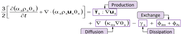
Figure 4: Granular temperature does not represent thermal heat; it is a mathematical equation that accurately calculates the kinetic bouncing energy of the solid particles.

When you set up your granular simulation in ANSYS Fluent, you must choose exactly how to mathematically solve this energy equation. You can choose the algebraic formulation, which solves much faster because it completely ignores how the energy diffuses and spreads out over space. Alternatively, you can choose to solve the full Partial Differential Equation (PDE). This full equation takes more time to calculate, but it tracks the exact transport and diffusion of the kinetic energy everywhere in the domain.

You must strictly select the full Partial Differential Equation (PDE) for granular temperature when your flow is highly rapid and complex, but you can safely use the faster algebraic form for simpler, steady-state flows.

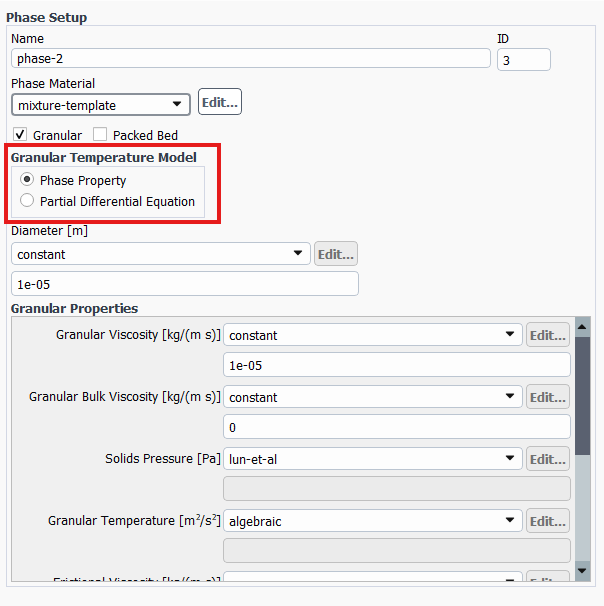
Figure 5: Two main approaches to granular temperature modeling

Solids Pressure

When you pump a heavy mixture of sand and water into a pipe, the solid sand particles constantly hit the pipe walls and violently crash into each other. This physical pushing force is called Solids Pressure. It is completely different from normal fluid pressure. It is a specific mathematical measurement of how much momentum is transferred when the hard solid spheres fly around and collide.

The software mathematically calculates this solids pressure by combining two different physical actions. The first part is the kinetic contribution, which happens when the particles fly freely through the empty fluid and hit a surface. The second part is the collisional contribution, which happens when the solid particles physically crash directly into one another.

There is a very crucial physical rule regarding this pressure. When the solid particles pack completely tightly together, they reach their absolute maximum volume fraction. At this exact packing limit, the granular flow becomes completely incompressible, exactly like tightly packed dirt. Because the particles cannot squeeze any closer together, the solids pressure mathematically spikes to an extreme level. This massive pressure spike is exactly what pushes the particles apart and strictly stops them from physically overlapping in your simulation.

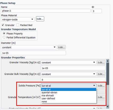
Figure 6: Available Solid pressure models in ANSYS Fluent

Inside ANSYS Fluent, you have three highly scientific models to calculate this pushing force. Here is a quick guide table to help you choose the exact proper model for your specific project:

Solids Pressure Model	Mathematical Approach	When to Choose This Model
Lun et al.	Calculates both the free-flight (kinetic) momentum and the crashing (collisional) momentum.	Best for general cases. Use this for standard fluidized beds where particles rapidly fly freely and crash frequently.
Syamlal et al.	Calculates ONLY the crashing (collisional) momentum. It completely ignores the free-flight energy.	Best for very dense flows. Use this when your particles are very heavy and constantly touching, with almost zero free flight.
Ma and Ahmadi	Calculates the kinetic and collisional forces, but also includes heavy frictional viscosity effects.	Best for packed beds. Use this for tightly packed geometries where heavy physical sliding and friction dominate the flow.

 

Model	Governing Equation
Lun et al.
Syamlal et al.
Ma and Ahmadi

 

Radial Distribution Function

In the Eulerian Granular Model, solid particles act very differently when they are flying far apart versus when they are crushed tightly together. When particles get very close to their maximum packing limit, the empty physical space between them almost completely disappears. Because they are forced into such a tight space, the physical probability of them violently crashing into each other increases massively. To accurately calculate this extreme collision rate, the software uses the Radial Distribution Function.

This mathematical concept acts as a powerful statistical multiplier in your governing equations. It automatically corrects the math and drastically increases the probability of particle collisions as the solid volume fraction gets denser. If you ignore this correction factor, your software will completely underestimate how often densely packed particles hit each other. You must strictly use a radial distribution function to mathematically prevent your solid particles from artificially overlapping and to calculate the correct heavy collision forces near the packing limit.

ANSYS Fluent provides four different mathematical models to calculate this exact collision probability. To help you easily choose the best one for your specific engineering project, please use the quick guide table below.

Radial Distribution Model	Quick Guide for Choosing the Proper Model
Lun et al.	The standard and most widely used general-purpose model. It works perfectly for most standard granular flows and is an excellent starting point.
Syamlal-O’Brien	The best choice when you are simulating bubbling or settling fluidized beds. It is highly recommended to use this exactly alongside the Syamlal-O’Brien drag model.
Ma and Ahmadi	The proper choice for extremely dense and heavy flows. It works perfectly when you also select the Ma and Ahmadi solids pressure model to include high frictional effects.
Arastoopour	A great alternative mathematical option for highly dense flows. It provides a very smooth numerical transition as the particles safely reach their absolute maximum packing limit.

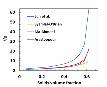
Figure 7: The radial distribution function is a mathematical multiplier that strictly increases the probability of particle collisions as they get dangerously close to their maximum packing limit.

Granular Viscosity

Just like thick honey resists flowing much more than liquid water, a moving mass of solid particles also heavily resists being pushed. This physical internal flow resistance is called Granular Viscosity. The software mathematically calculates this total flow resistance by strictly adding three completely different physical mechanisms together.

The first mechanism is the kinetic viscosity, which measures the resistance created when particles fly freely across the flow streams. The second mechanism is the collisional viscosity, which measures the heavy friction caused when particles directly crash and bounce off each other. The third and final mechanism is the bulk viscosity, which calculates how much the entire cloud of particles physically resists being compressed or expanded as a whole volume.

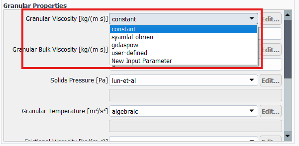
Figure 10: Available Granular viscosity models in ANSYS Fluent

Inside ANSYS Fluent, you must select exactly how to calculate these viscous forces. Here is a quick guide table to help you choose the proper kinetic granular viscosity model:

Granular Viscosity Model	Mathematical Approach	When to Choose This Model
Lun et al.	Calculates both kinetic and collisional viscosity simultaneously.	Best for standard flows. This is the default and most robust choice for general fluid-solid interactions and bubbling beds.
Syamlal et al.	A specialized kinetic viscosity calculation.	Best for uniform math. Use this specifically when you have chosen Syamlal et al. for your other models to maintain numerical stability.
Gidaspow et al.	An advanced kinetic viscosity calculation.	Best for dense fluidized beds. Highly recommended for flows where particles frequently alternate between flying freely and packing tightly.

 

Frictional Stress Modeling

When solid particles are flowing freely in a dilute mixture, they simply bounce and crash into each other. However, as the particles accumulate at the bottom of a tank or inside a hopper, they eventually run out of empty space to fly.

When the volume fraction of the solids reaches the critical packing limit of 0.63, the physical behavior of the flow changes completely. At this extreme density, the particles can no longer bounce freely. Instead, they are forced into constant physical contact and begin heavily sliding, grinding, and rubbing directly against one another.

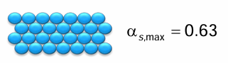
To accurately capture this intense grinding motion, the software must completely stop relying on collision physics and start using soil mechanics. It activates Frictional Stress Modeling, which calculates the heavy mechanical friction created by the sliding particle surfaces.

This heavy frictional stress is mathematically divided into two parts: frictional pressure and frictional viscosity. When your solids volume fraction exceeds the packing limit, the software strictly adds these massive frictional forces to the total solid stress to prevent the simulation from failing. ANSYS Fluent provides a few specialized mathematical models to accurately calculate this heavy sliding friction. Here is a quick guide table to help you easily choose the exact proper frictional model for your specific dense flow:

Frictional Model	Mathematical Approach	When to Choose This Model
Schaeffer (Coulomb Law)	Calculates pure sliding frictional viscosity based directly on the internal friction angle of the solids.	Best for standard packed flows. Use this as your default choice for hoppers, silos, and deeply settled beds.
Johnson and Jackson	A comprehensive model that mathematically calculates both frictional pressure and frictional viscosity.	Best for heavy soil mechanics. Highly recommended when simulating extremely heavy, dirt-like sliding flows where particles are totally locked.
Syamlal et al.	Calculates frictional pressure using specific volume fraction curves.	Best for consistent Syamlal setups. Use this specifically to maintain numerical stability if you have already chosen Syamlal for your drag or collision models.

 

Drag Models for Gas-Solid Flows

When a fluid flows through a cloud of solid particles, the gas physically grabs the solid spheres and pushes them forward. This aerodynamic pulling force is called Interphase Drag. In a highly dilute flow, a single particle flies freely and experiences a standard, predictable drag resistance. However, when thousands of particles fly tightly together, they create complex drafting effects, change the flow shape, and severely block the gas pathways.

Because of this heavy crowding effect, the software cannot simply use standard single-particle equations. It must use specialized gas-solid drag models that mathematically increase the friction based on exactly how densely the particles are packed.

Choosing the exact proper drag model is the absolute most critical step to correctly predict terminal velocities in dilute pipes and minimum fluidization velocities in dense beds.

ANSYS Fluent provides several highly specialized mathematical equations to calculate this gas-solid friction. Because drag strongly depends on the particle diameter and concentration, you must select the model that matches your flow regime.

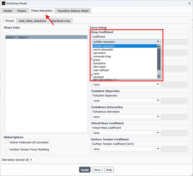
Figure 11: Drag models for granular flows in ANSYS Fluent

Here is a quick guide table to help you perfectly choose the exact proper gas-solid drag model for your simulation:

Gas-Solid Drag Model	Mathematical Approach	When to Choose This Model
Wen and Yu	An extension of standard single-particle drag, corrected for slightly crowded spaces.	Best for dilute systems. Use this when your flow is mostly empty gas with light particle dispersion.
Gidaspow	Strictly combines the Wen-Yu model for dilute zones and the heavy Ergun equation for densely packed zones.	Best for dense fluidized beds. The most highly recommended standard choice for heavy gas-solid interactions.
Huilin-Gidaspow	Uses the exact same equations as Gidaspow but adds a specialized mathematical blending function.	Best for mixed flows. Use this to prevent numerical crashes when your flow rapidly transitions between highly dense and completely dilute.
Syamlal-O’Brien	Mathematically adjusts the drag friction based specifically on the terminal velocity of settling particles.	Best for bubbling beds. Highly recommended when you already know your exact minimum fluidization velocity.
Gibilaro	Uses theoretical considerations to calculate the pressure drop across moving and expanding beds.	Best for circulating beds. Gives highly accurate predictions for turbulent bed expansion.

 

Interphase Heat Transfer for Granular Flows

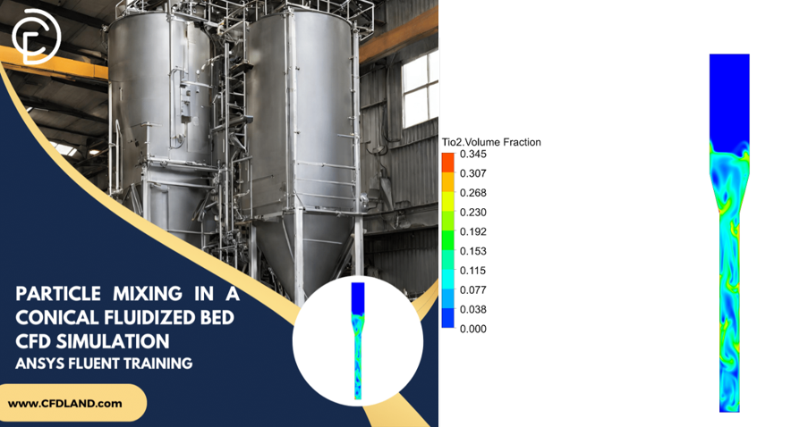
In many multiphase applications, the fluid and solid phases enter the system at completely different temperatures. As they mix and interact, thermal energy is constantly exchanged between them until they reach an equilibrium. This thermal exchange is known as interphase heat transfer. Accurately predicting this temperature shift is essential for simulating complex thermal processes like drying, combustion, or catalytic reactions. You can explore a great example of complex particle dynamics and mixing in our Particle Mixing in a Conical Fluidized Bed CFD Simulation, ANSYS Fluent Training tutorial.

ANSYS Fluent manages this thermal exchange through the Phase Interaction panel. By defining a volumetric heat transfer coefficient, the software can calculate exactly how fast heat moves from the continuous fluid to the dispersed particles, or vice versa. Because different flow regimes and particle types transfer heat at very different rates, Fluent offers a wide variety of empirical models to calculate this coefficient. Choosing the correct model depends heavily on whether you are simulating solid particles, liquid droplets, or gas bubbles.

Below is a comprehensive quick-guide table detailing all the available heat transfer coefficient models in ANSYS Fluent and when to use them for your specific project:

Heat Transfer Model	Description & Best Use Case
gunn	Best for Granular Flows. This model is specifically designed and frequently used for Eulerian multiphase simulations involving a solid granular phase, making it the top choice for fluidized beds.
ranz-marshall	Best for Droplets/Bubbles. This model is frequently used for Eulerian multiphase simulations that do not involve a granular phase, such as liquid droplets in a gas.
hughmark	Best for High-Speed Droplets/Bubbles. This is an extension of the Ranz-Marshall model designed to remain accurate over a much wider range of Reynolds numbers.
tomiyama	Best for Slow Bubbles. This model is frequently used for Eulerian multiphase simulations of bubbly flows operating at relatively low Reynolds numbers.
constant-htc	Best for Simplified Thermal Models. This allows you to specify a fixed, constant value for the volumetric heat transfer coefficient if you already know the exact exchange rate.
nusselt-number	Best for Known Empirical Data. This allows you to specify a constant value for the Nusselt number, from which the software will automatically compute the heat transfer coefficient.
fixed-to-sat-temp	Best for Simple Phase Change. This models heat transfer when all heat transferred to an interface is used in mass transfer, assuming the destination phase remains at the saturation temperature.
two-resistance	Best for Evaporation-Condensation. This opens a secondary dialog box allowing you to independently specify the heat transfer coefficient correlations for both the liquid and gas phases.
time-scale (two-resistance sub-model)	Best for Rapid Phase Change. This models the gas-interface heat transfer by assuming the gas phase retains the saturation temperature through rapid evaporation or condensation.
zero-resistance (two-resistance sub-model)	Best for Interfacial Equilibrium. When selected for one of the phases, it forces that specific phase’s temperature to be exactly equal to the interfacial temperature.
user-defined	Best for Custom Research. This allows you to hook a User-Defined Function (UDF) to implement a custom correlation for the heat transfer coefficient.
none	Best for Isothermal Flows. This instructs the solver to completely ignore the effects of heat transfer between the two phases.

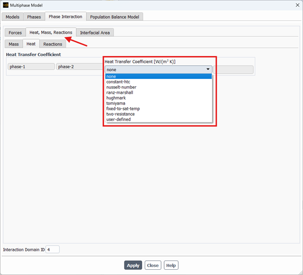
Figure 12: ANSYS Fluent provides a wide variety of heat transfer coefficient models in the Phase Interaction panel to accurately simulate thermal exchange between different phases.

 

Eulerian Granular Model Setup in Fluent

Setting up a standard multiphase simulation in ANSYS Fluent is relatively straightforward. However, when your solid particles reach high concentrations, you must explicitly instruct the software to activate the complex soil mechanics and kinetic theory equations. To do this, you must navigate to the Phases panel and edit your secondary solid phase. By checking the Granular option inside the secondary phase dialog box, you immediately unlock a completely new set of specialized mechanical properties.

The software will now require you to mathematically define exactly how the particles bounce, slide, flow, and pack together. Instead of just entering a simple density and viscosity, you must carefully assign specific models for the granular temperature, internal friction, and solid pressure.

Failing to define these granular parameters correctly will cause your dense particle bed to either artificially collapse into a tiny volume or explode with numerical instability. To guarantee a successful simulation, you must set up the secondary phase properties correctly.

 

Packed Bed Simulation

In many heavy chemical engineering applications, such as catalytic reactors, thermal energy storage, or filtration systems, the solid particles do not move at all. Instead, they sit completely stationary in a dense, tightly locked column while the fluid flows rapidly through the tiny gaps between them.

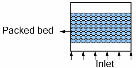
Traditionally, engineers simulate these complex stationary zones using a simplified Porous Media model. We have successfully utilized this macroscopic approach in several of our advanced projects. For example, in our Heat Transfer from Cylinder in Porous Medium CFD Simulation, we treated an entire packed bed as a porous zone using the Darcy-Brinkman-Forchheimer formulation. This simplified the geometry and perfectly validated forced convection without the computationally impossible task of meshing millions of individual particles.

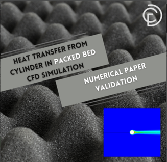
Figure 13: An application of porous media for modeling packed bed

While the porous media approach is excellent for simple flow resistance, ANSYS Fluent also allows you to use the Eulerian Granular model to create a much more detailed, physics-based packed bed. This Eulerian approach is mathematically the absolute best physical representation of stationary particles because it actively calculates the true interphase drag, solids pressure, and local volume fractions.

By using the Eulerian packed bed approach instead of a simple porous zone, you gain full, unrestricted access to the advanced homogeneous and heterogeneous reactions framework to simulate complex surface chemistry.

Setting up an Eulerian packed bed requires a very specific two-step process in the software. First, you must edit your secondary solid phase, enable the Granular option, and explicitly check the Packed Bed box to activate the specialized stationary equations. Second, you must navigate to the Cell Zone Conditions panel and manually set the packed solids velocity components to exactly zero. This effectively freezes the particles in place, forcing the continuous fluid to strictly navigate through the tightly locked solid structure.

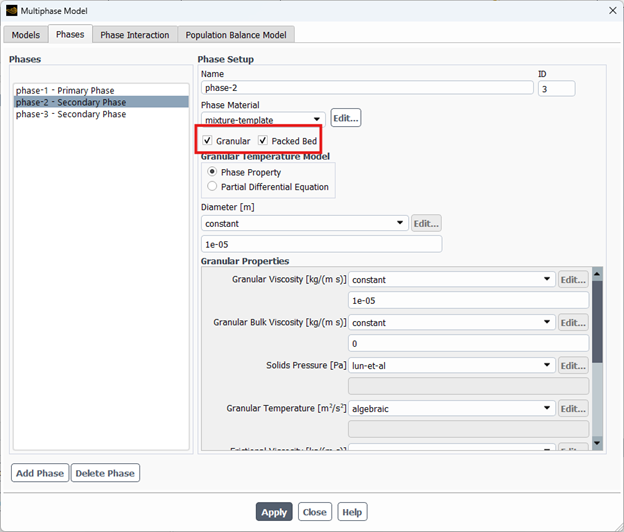
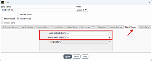
Figure 14: Simulating a packed bed using the Eulerian Granular model provides a superior physical representation of stationary particles and unlocks advanced heterogeneous reaction capabilities.

Conclusion

To wrap up this comprehensive guide, we have thoroughly explored the powerful physics behind the Eulerian Granular Model in ANSYS Fluent. From understanding the advanced gas-solid drag equations to correctly freezing particles for a stationary packed bed, you now have the exact foundational knowledge required to simulate heavy, dense particulate flows.

Remember, choosing the proper interphase momentum and heat transfer models is the absolute key to preventing numerical instability and achieving highly realistic, data-driven simulations.

Whether you are designing bubbling fluidized beds, circulating reactors, or complex filtration systems, mastering these granular setups will drastically elevate the accuracy of your engineering projects. You can explore our extensive library of prepared Multiphase CFD Simulation Tutorials to see these exact Eulerian settings applied step-by-step in real industrial cases.