
A heat exchanger is a device that transfers heat between a hot fluid and a cold fluid without mixing them. Heat exchangers are widely used in power plants, HVAC systems, chemical processes, and thermal engineering applications.

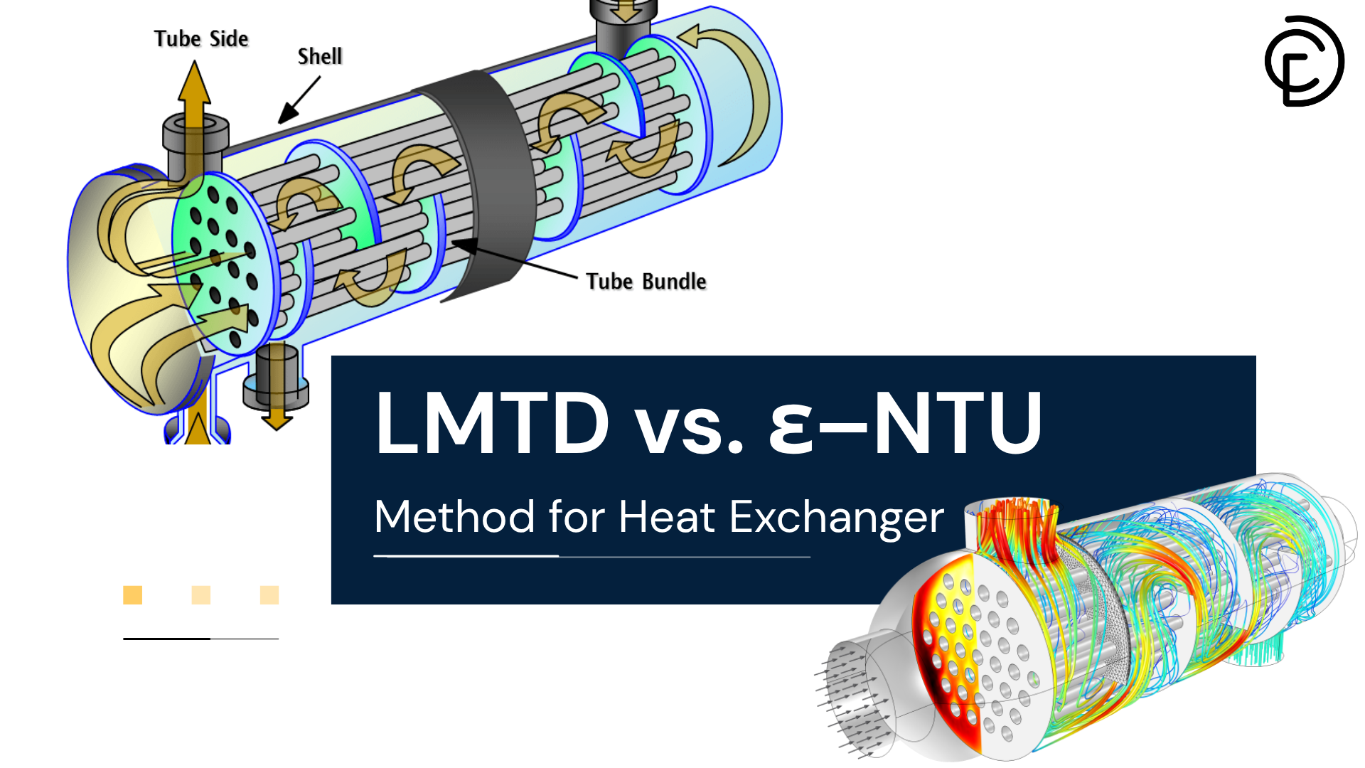
Figure 1: The wide range of applications of heat exchangers in numerical analysis and the use of methods LMTD and ε–NTU. You can find more on our Heat Exchanger CFD Tutorials Library
In heat exchanger analysis, engineers are mainly interested in design and performance. These two tasks appear in almost all practical engineering problems.
Heat exchanger analysis problems usually involve two main goals:
- Selecting a heat exchanger that can produce a required temperature change for a fluid with a known mass flow rate.
- Predicting the outlet temperatures of the hot and cold fluids for a given heat exchanger.
These two goals form the basis of all heat exchanger design and performance calculations.
Steady‑State Heat Exchanger Behavior
Most heat exchangers operate for long periods with almost constant operating conditions. Because of this, a heat exchanger can be modeled as a steady‑flow device.
Under steady conditions:
- Mass flow rates are constant
- Inlet and outlet temperatures do not change with time
- Heat transfer rate is constant
This assumption simplifies thermal analysis of heat exchangers and is widely used in engineering design and CFD simulations.
Energy Balance for Hot and Cold Fluids
An overall energy balance can be applied separately to the hot fluid (h) and the cold fluid (c).
For the hot fluid:

For the cold fluid:

Where:
- m˙ is the mass flow rate
- cp is the specific heat
- i and o denote inlet and outlet
These equations show that the same heat transfer rate q links the hot and cold sides of the heat exchanger.
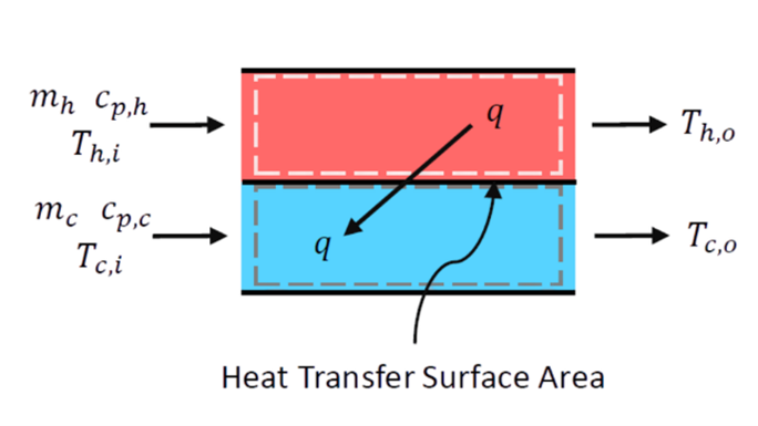
Figure 2: Section of a Parallel Flow Heat Exchanger, Which basically describes the input and output variables.
Need for a Mean Temperature Difference
The temperature difference between the hot and cold fluids is defined as:

However, this temperature difference changes along the length of the heat exchanger. It is not constant.
Because of this variation, heat transfer cannot be calculated using a simple temperature difference. Instead, a mean temperature difference must be used.
This leads to the general heat transfer rate equation:

Where:
- U is the overall heat transfer coefficient
- A is the heat transfer surface area
- ΔTₘ is the appropriate mean temperature difference
Choosing the correct form of ΔTₘ is the key point in heat exchanger analysis.
Two Main Analysis Methods
Based on how the temperature difference is handled, two main methods are used in heat exchanger analysis:
- Log Mean Temperature Difference (LMTD) method
- Effectiveness–NTU (ε–NTU) method
The LMTD method is best when inlet and outlet temperatures are known.
The ε–NTU method is best when only inlet temperatures are known.
These two methods form the foundation of heat exchanger design, performance evaluation, and CFD-based thermal analysis.
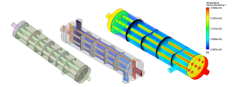
Figure 3: heat exchanger concept with hot (h) and cold (c) fluid streams.
Heat Exchanger Flow Arrangements and Temperature Profiles
The flow arrangement of a heat exchanger describes how the hot and cold fluids move relative to each other. This arrangement strongly affects the temperature profiles, the mean temperature difference, and the overall heat transfer performance.
In heat exchanger analysis, the most common flow arrangements are:
- Parallel flow
- Counterflow
- Crossflow
Understanding these arrangements is essential for both heat exchanger design and performance analysis.
Parallel Flow Heat Exchanger
In a parallel flow heat exchanger, the hot and cold fluids enter at the same end and flow in the same direction.
At the inlet:
- The temperature difference between the fluids is maximum
- Heat transfer is very strong near the entrance
Along the length:
- Both fluid temperatures change rapidly
- The temperature difference decreases quickly
The temperature difference at any location is defined as:
For a parallel flow heat exchanger, the endpoint temperature differences are:


Because the temperature difference drops fast, parallel flow heat exchangers are less thermally efficient than counterflow units.
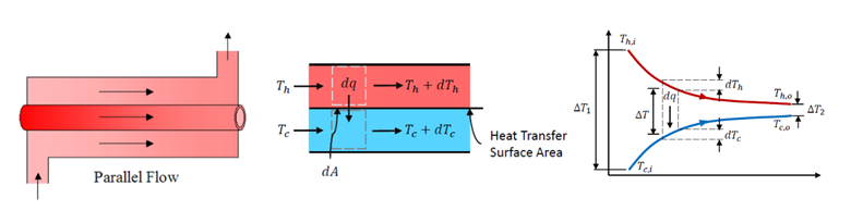
Figure 4: Temperature profiles of hot and cold fluids in a parallel flow heat exchanger. Both fluids enter at the same end, causing a large temperature difference near the inlet.
Counterflow Heat Exchanger
In a counterflow heat exchanger, the hot and cold fluids enter from opposite ends and flow in opposite directions.
This arrangement creates:
- A more uniform temperature difference
- A higher log mean temperature difference (LMTD)
For a counterflow heat exchanger, the endpoint temperature differences are:
The LMTD of a counterflow heat exchanger is always higher than that of a parallel flow heat exchanger.
Because of this:
- Less heat transfer area is required
- Counterflow heat exchangers are preferred in engineering practice
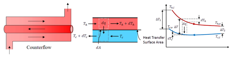
Figure 5: Temperature profiles in a counterflow heat exchanger. Opposite flow directions produce a more uniform temperature difference and higher thermal efficiency.
Crossflow Heat Exchanger
In a crossflow heat exchanger, the hot and cold fluids move approximately perpendicular to each other.
Crossflow arrangements are common in:
- Air coolers
- Radiators
- Compact heat exchangers
Because the temperature distribution is more complex:
- A simple LMTD expression is difficult
- A correction factor (F) is often required
- The ε–NTU method is frequently preferred
Crossflow heat exchangers are widely analyzed using effectiveness–NTU relations instead of direct LMTD formulas.
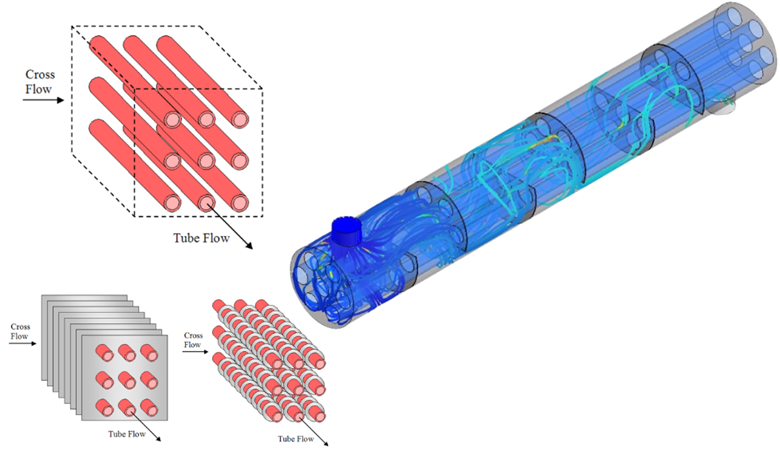
Figure 6: Crossflow heat exchanger configuration showing perpendicular motion of hot and cold fluids, commonly used in air to fluid applications.
Temperature Profiles and Engineering Insight
The temperature profile shows how fluid temperatures change along the heat exchanger length. It explains:
- Why the temperature difference is not constant
- Why a mean temperature difference is required
|
large inlet temperature difference, rapid decay |
|
nearly uniform temperature difference |
|
complex temperature field |
Flow arrangement directly controls thermal efficiency, required area, and heat exchanger performance.
Log Mean Temperature Difference (LMTD) Method
The Log Mean Temperature Difference (LMTD) method is one of the most important tools in heat exchanger analysis. It is mainly used for design and performance calculations when the inlet and outlet temperatures of both fluids are known.
In this method, the heat transfer rate is written as:

Where:
- q is the total heat transfer rate
- U is the overall heat transfer coefficient
- A is the heat transfer surface area
- ΔTm is the mean temperature difference
Why a Mean Temperature Difference Is Needed? In a heat exchanger, the temperature difference between the hot and cold fluids is not constant. It changes along the flow direction. The local temperature difference is defined as:
Because this difference varies with position, a simple average temperature difference cannot be used. A special mean value is required. This leads to the log mean temperature difference, or LMTD. The LMTD represents the true thermal driving force for heat transfer.
Consider a differential element of a heat exchanger with area dA. For the hot fluid:

For the cold fluid:

The heat transfer across the surface is:

Where:
Combining these relations and integrating along the heat exchanger length leads to the log mean temperature difference expression.
LMTD Formula: The log mean temperature difference is defined as:

Where:
- ΔT1 and ΔT2 are the temperature differences at the two ends of the heat exchanger
The heat transfer rate becomes:

- LMTD for Parallel Flow Heat Exchangers
In a parallel flow heat exchanger, both fluids enter at the same end. The temperature differences are defined as:


For parallel flow, the temperature difference decreases rapidly along the length. Parallel flow heat exchangers generally have a lower LMTD.
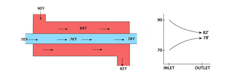
Figure 7: A simple example of temperature changes in Parallel flow heat exchanger.
- LMTD for Counterflow Heat Exchangers
In a counterflow heat exchanger, the fluids move in opposite directions. The temperature differences are:
For the same inlet and outlet temperatures:

Counterflow heat exchangers require a smaller heat transfer area for the same heat duty.
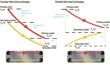
Figure 8: Temperature profiles and decreasing temperature difference in a parallel flow heat exchanger, Higher and more uniform temperature difference in a counter-flow heat exchanger.
Correction Factor for Complex Heat Exchangers
The basic LMTD relation is exact only for:
- Parallel flow
- Counterflow
For crossflow and multi‑pass shell‑and‑tube heat exchangers, a correction factor F is used:

Where:
- is the counterflow LMTD
- F≤1
- F=1 corresponds to an ideal counterflow exchanger
The correction factor depends on:
- Heat exchanger geometry
- Inlet and outlet temperatures of hot and cold fluids
The correction factor measures the deviation from ideal counterflow behavior.
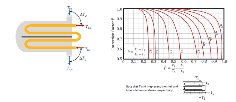
Figure 9: Correction factor F as a function of temperature ratios and heat exchanger configuration.
The LMTD method is widely used as a reference model in CFD simulations of heat exchangers. A good example is the Spiral Heat Exchanger CFD Simulation provided by CFD Land:
In this example:
- Hot and cold fluids flow through spiral channels, typically in a counterflow arrangement
- Inlet and outlet temperatures are specified
- The heat transfer coefficient and heat transfer rate are obtained using ANSYS Fluent
- The LMTD method provides the theoretical basis for validating CFD results
Such CFD simulations use the LMTD method to connect numerical results with classical heat exchanger theory.
- ANSYS Fluent heat transfer simulations
- Thermal performance evaluation
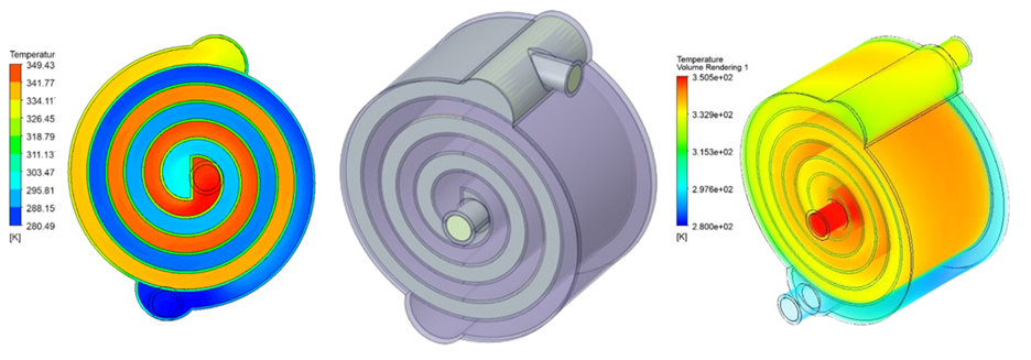
Figure 10: the Spiral Heat Exchanger CFD Simulation provided by CFDLAND, CFD simulations use the LMTD method
Effectiveness–NTU (ε–NTU) Method
The Effectiveness–NTU (ε–NTU) method is widely used in heat exchanger analysis when the outlet temperatures of the fluids are unknown. In such cases, using the LMTD method requires iteration, which is not efficient. The ε–NTU method avoids this problem by using dimensionless parameters and is therefore preferred for heat exchanger design and performance prediction.
Heat Exchanger Effectiveness
The effectiveness (ε) of a heat exchanger is defined as the ratio of the actual heat transfer rate to the maximum possible heat transfer rate.

The actual heat transfer rate is:

The maximum possible heat transfer occurs when the fluid with the minimum heat capacity rate experiences the maximum temperature difference:

Where:


Effectiveness measures how close a real heat exchanger is to ideal performance.
Number of Transfer Units (NTU)
The Number of Transfer Units (NTU) is a dimensionless parameter that represents the size and thermal strength of a heat exchanger.

Where:
- U is the overall heat transfer coefficient
- A is the heat transfer surface area
A higher NTU means:
- Larger heat transfer area
- Higher effectiveness
General ε–NTU Relation
For any heat exchanger, effectiveness is a function of:

The heat transfer rate can then be calculated directly as:

This allows direct calculation of heat transfer rate and outlet temperatures without iteration.
ε–NTU Relations for Common Flow Arrangements
The effectiveness depends strongly on the flow arrangement.
From the file, the most important relations are:
- Parallel flow
![\varepsilon = \left( \frac{1 - \exp[-NTU(1 + C_r)]}{1 + C_r} \right)](https://cfdland.com/wp-content/ql-cache/quicklatex.com-67439d85ced4a3e331204a743c885f13_l3.png "Rendered by QuickLaTeX.com")
- Counterflow
![\varepsilon = \frac{1 - \exp[-NTU(1 - C_r)]}{1 - C_r \exp[-NTU(1 - C_r)]}, (C_r \neq 1)](https://cfdland.com/wp-content/ql-cache/quicklatex.com-b218f86deede3ff97ab3604a37977901_l3.png "Rendered by QuickLaTeX.com")
Where:

Counterflow heat exchangers always give higher effectiveness than parallel flow for the same NTU.
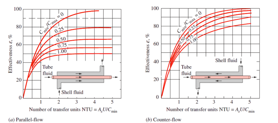
Figure 11: Variation of heat exchanger effectiveness with NTU for different flow arrangements
Special Case: Condensers and Boilers
In condensers and boilers, one fluid undergoes a phase change.
During phase change:
- Temperature remains almost constant
- Heat capacity rate becomes very large

For this case: 
This assumption is commonly used in condenser CFD simulations and boiler thermal design.
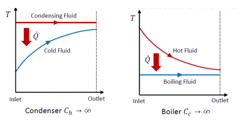
Figure 12: Heat exchangers with phase change, where one fluid remains at nearly constant temperature.
Design and Performance Use
From the file, the ε–NTU method is used in two main ways:
- Design problem
- Inlet temperatures and flow rates known
- Required outlet temperatures specified
- NTU is calculated first
- Heat transfer area A is determined
- Performance problem
- Existing heat exchanger
- NTU and effectiveness calculated
- Heat transfer rate and outlet temperatures predicted
This makes the ε–NTU method ideal for both heat exchanger design and evaluation.
LMTD vs. ε–NTU: Practical Use and Limitations
The LMTD method and the ε–NTU method are the two standard tools for heat exchanger analysis. Both are based on the same energy balance, but they are used in different engineering situations.
Practical Use in Engineering
The LMTD method is best suited for design problems where:
- Inlet and outlet temperatures of both fluids are known
- The required heat transfer area must be calculated
This agrees with the file, which states that LMTD is ideal when the temperature change is specified.
The ε–NTU method is best suited for performance problems where:
- Only inlet temperatures are known
- Outlet temperatures must be predicted
- A real heat exchanger is already selected
Table 1: Key Practical Differences
| Aspect | LMTD Method | ε–NTU Method |
| Main use | Design (area sizing) | Performance prediction |
| Known temperatures | Inlet + outlet | Inlet only |
| Iteration needed | Yes (if outlets unknown) | No |
| Flow arrangement | Simple (PF, CF) | All types |
| CFD validation | Very common | Less direct |
Table 2: Main Limitations of LMTD and ε–NTU method
| Limitations of the LMTD method | Limitations of the ε–NTU method |
| Not convenient when outlet temperatures are unknown | Requires estimation of U and Cₘᵢₙ
|
| Requires a correction factor (F) for crossflow and multipass exchangers | Effectiveness relations depend on exchanger type
|
| Less flexible for complex geometries
|
Less intuitive temperature interpretation
|

Figure 13: Strengths of each method
Both methods are complementary, not competing.
In real projects:
- Engineers often start with ε–NTU
- Final sizing and verification are done using LMTD
When to Use LMTD vs. ε–NTU (Quick Engineering Guide)
The choice between the LMTD method and the ε–NTU method depends mainly on which temperatures are known and what type of problem is being solved.
Table 3: Quick Selection Guide
| Engineering Situation | Recommended Method | Reason |
| Inlet and outlet temperatures known | LMTD method | Direct and simple |
| Only inlet temperatures known | ε–NTU method | No iteration required |
| Heat exchanger sizing (area needed) | LMTD method | Design‑oriented |
| Existing exchanger performance | ε–NTU method | Rating‑oriented |
| Counterflow / parallel flow | LMTD or ε–NTU | Both applicable |
| Crossflow or multipass exchangers | ε–NTU method | More flexible |
| CFD validation studies | LMTD method | Clear physical meaning |
This table is the fastest way to choose the correct heat exchanger analysis method in practice.
Design vs. Performance Procedure
- Design Procedure (Sizing a Heat Exchanger)
Goal:
Select a heat exchanger type and determine the required heat transfer area.
Typical inputs:
- Inlet temperatures

- Desired outlet temperatures

- Mass flow rates

Procedure:
- Calculate heat capacity rates:
- Determine: Cmin & Cmax
- Compute effectiveness: epsilon
- Use ε–NTU relations to find: NTU
- Calculate required area:

Most commonly uses the ε–NTU method
- Performance Procedure (Rating a Heat Exchanger)
Goal:
Evaluate an existing heat exchanger and predict outlet temperatures.
Typical inputs:
- Inlet temperatures
- Mass flow rates
- Known exchanger area: A
Procedure (from the file):
- Calculate NTU:
- Find effectiveness: epsilon
- Compute heat transfer rate:
- Determine outlet temperatures:
Most commonly uses the ε–NTU method
LMTD can be used if outlet temperatures are already known
CFD Post‑Processing Validation Using LMTD and ε–NTU Methods
In CFD simulations of heat exchangers, numerical results must be validated to ensure physical correctness.
This validation is usually done in post‑processing by comparing CFD data with analytical or numerical solutions based on LMTD and ε–NTU methods.
Validation Concept
From the lesson file, heat exchanger behavior is governed by the energy balance:
In CFD:
- Temperatures are extracted at inlets and outlets
- Mass‑averaged values are used
- Heat transfer rate is calculated numerically
The same quantities are then computed using classical heat exchanger formulas.
Agreement between CFD and analytical results validates the simulation.
LMTD‑Based Validation
Using CFD results:
- Extract:

- Compute endpoint temperature differences:

- Calculate:

- Compare:
![\varepsilon_{CFD} [latex] vs. [latex] q_{LMTD} = U A \Delta T_{lm}](https://cfdland.com/wp-content/ql-cache/quicklatex.com-4d4c6befd05c93305ef46bdca8a2f769_l3.png "Rendered by QuickLaTeX.com")
A small difference confirms correct thermal behavior and boundary conditions.
ε–NTU‑Based Validation
Alternatively, validation can be done using effectiveness:

From theory: 
Comparing: 
confirms the accuracy of heat transfer prediction.
Engineering Insight
- LMTD is often used to validate overall heat transfer rate
- ε–NTU is useful when outlet temperatures are uncertain
- Both methods are consistent with steady‑state CFD simulations
These validation steps directly link CFD post‑processing with classical heat exchanger theory.
A useful practical example is the Spiral Heat Exchanger CFD Simulation Considering Heat Transfer Coefficient – ANSYS Fluent Training from CFDLAND. This tutorial is relevant because spiral heat exchangers are commonly evaluated by comparing numerical CFD results with heat transfer relations such as the LMTD method and, in design studies, the ε–NTU method.
This kind of example helps connect:
- heat exchanger theory
- CFD post-processing
- ANSYS Fluent validation
- practical engineering design
This example shows how classical heat exchanger methods and CFD simulation can support each other in real engineering work.

Figure 14: Spiral heat exchanger CFD training from cfdland. This example connects ANSYS Fluent simulation with practical heat exchanger analysis and validation.
Conclusion
In this article, we reviewed the fundamentals of heat exchanger analysis with a clear focus on design and performance calculations. Heat exchangers usually operate under steady‑flow conditions, which allows the use of simplified and reliable thermal models.
Two classical and widely accepted methods were discussed:
- The Log Mean Temperature Difference (LMTD) method, which is best suited for design problems where inlet and outlet temperatures are known and the required heat transfer area must be determined.
- The Effectiveness–NTU (ε–NTU) method, which is best suited for performance analysis where only inlet temperatures are known and outlet temperatures must be predicted.
The article also showed that flow arrangement (parallel flow, counterflow, crossflow) has a strong effect on temperature profiles, thermal efficiency, and required surface area. For complex geometries, the use of a correction factor or ε–NTU relations becomes necessary.
Finally, the design vs. performance procedure was clarified:
- Design calculations are used for custom heat exchanger sizing.
- Performance calculations are used to evaluate existing or vendor‑supplied heat exchangers.
LMTD and ε–NTU are not competing methods. They are complementary tools that engineers must choose based on available data and design goals.
These methods form the theoretical foundation for modern CFD simulations, ANSYS Fluent heat transfer analysis, and practical heat exchanger engineering.