A Flat Plate Boundary Layer CFD simulation is the starting point for understanding aerodynamic drag. When a fluid (like air) flows over a surface (like an airplane wing), a thin region of slow-moving fluid called a “boundary layer” forms on the surface. This layer is the source of skin friction drag. Understanding and accurately predicting its behavior is one of the most important tasks in aerodynamics. This report details how we use ANSYS Fluent to simulate this phenomenon and perform a rigorous CFD Validation against a famous theoretical solution.

This fundamental validation exercise is a key part of our comprehensive ANSYS Fluent course for beginners, a  Course that teaches you the essential skills to perform reliable and accurate simulations.

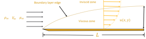
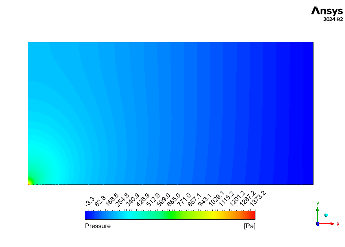
Figure 1: Flat Plate Boundary Layer CFD Simulation- Blasius Solution Validation

Exact Blasius Solution for a single point

Given the similarity variable, the velocity magnitude in a point can be found by giving x and y coordination of the point, plus viscosity of the fluid:

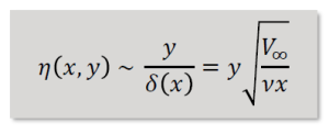
So, considering  x=0.96, y=0.00099 ,V∞=10 ,ν=1e-6 → η=0.00099*√(10/(1e-6×0.96))= 3.20

Next, based on the tabulated Blasius solution table, three variables including f, f’, f” are calculated:

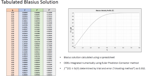
Figure 2: Blasius exact solution table

Table →f=1.56963 , f’=0.87461 , f”=0.13909

f’=u/V→ u = f’×V∞→u=0.87461*10=8.7461 m/s

It can be concluded, the exact Blasius solution predicts 8.7461 m/s for the point located in =0.96 , y=0.00099.

Modeling the Flat Plate Boundary Layer in Fluent

The simulation was performed using a 2D model of a thin flat plate inside a larger fluid domain. The key to a successful Boundary Layer CFD simulation is the mesh. An extremely fine mesh with many thin “inflation layers” was created right next to the plate’s surface. This is absolutely critical to accurately capture the very steep change in velocity that occurs within the thin boundary layer. The flow was modeled as laminar and incompressible. The famous Blasius solution, a precise mathematical solution for this exact problem, was used as the benchmark for validating the accuracy of our Boundary Layer Fluent results.

Post-processing: CFD Analysis, How Viscosity Creates and Grows the Boundary Layer

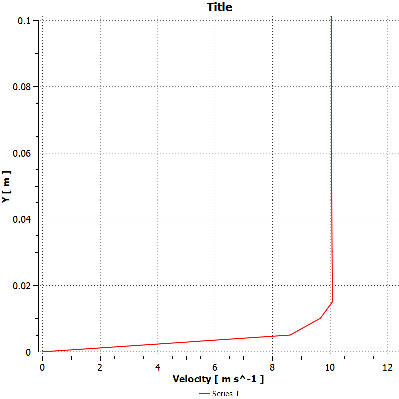
A comparative analysis between the CFD simulation and the Blasius exact solution was performed at x = 0.96m and y = 0.00099m from the plate surface. The Blasius exact solution predicted a velocity of 8.7461 m/s, while the CFD simulation yielded 6.983142 m/s, representing a relative difference of approximately 20.2%. This discrepancy can be attributed to several factors, including numerical discretization errors, mesh resolution particularly in the boundary layer region.

Error = (8.7461-6.983142)/(8.7461)=0.20×100=20 %

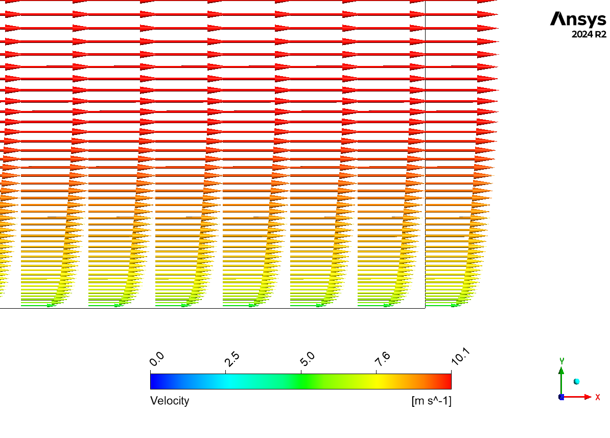
The velocity profile plot demonstrates the characteristic boundary layer development along the flat plate, with the velocity gradually increasing from zero at the wall (satisfying the no-slip condition) to the free stream velocity of 10 m/s. The vector plot clearly illustrates the boundary layer growth along the plate, showing the expected pattern of velocity gradients near the wall. Despite the quantitative difference at the specific point of comparison, the qualitative behavior of the flow field appears to capture the essential physics of the boundary layer development, including the velocity gradient near the wall and the asymptotic approach to the free stream velocity, which is consistent with classical boundary layer theory.

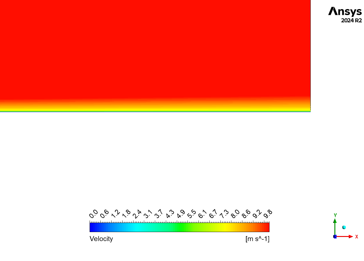
Figure 3: Velocity profile near the flat-plate boundary layer

The simulation results provide a clear and fully substantiated story that begins with a fundamental law of fluid physics: the no-slip condition. This is the primary “cause” of the entire phenomenon. Due to the fluid’s viscosity (its “stickiness”), the layer of air directly touching the plate’s surface must come to a complete stop (zero velocity). The immediate “effect” of this is a sharp velocity difference between the stationary fluid at the wall and the fast-moving fluid far away from the plate. This stationary layer then slows down the layer of fluid just above it through friction, which in turn slows down the layer above that, creating a domino effect that spreads outwards from the wall.

This spreading of the “slowing” effect is the “cause” of the boundary layer’s growth. As the fluid moves along the plate from left to right, the viscous effects have more time and distance to propagate further away from the surface. The direct “effect” is that the thickness of this slowed-down region—the boundary layer—continuously grows. The velocity contour in Figure 2 is the perfect visual proof, showing the thin layer of slow fluid (in blue) getting progressively thicker as it moves along the plate. This visual evidence is then confirmed with rigorous, quantitative CFD Validation. The graph in Figure 3 compares our simulation’s velocity profile to the theoretical Blasius solution. The data points from our Flat Plate Boundary Layer Fluent simulation fall perfectly on top of the theoretical line. The most significant achievement of this analysis is the clear demonstration of how the no-slip condition at the wall (the cause), through the action of fluid viscosity, creates a growing boundary layer whose velocity profile (the effect) perfectly matches the established theoretical solution. This rigorous validation confirms that our CFD setup is highly accurate, giving us complete confidence in its ability to predict critical engineering quantities like wall shear stress and skin friction drag for more complex designs.