

Have you ever noticed how water flows smoothly from a slightly opened faucet but becomes chaotic when fully opened? This everyday observation demonstrates the fascinating difference between laminar and turbulent flow, two fundamental concepts in fluid dynamics that affect countless aspects of our world. In this comprehensive guide, we’ll explore the key characteristics that distinguish laminar vs turbulent flow, examine real-world examples of each, and explain how the Reynolds number helps us predict which type of flow will occur in different situations. Furthermore, we’ll look at how these concepts apply to natural settings like rivers and lakes, and how modern computational tools like ANSYS Fluent simulate these flow patterns.
Whether you’re studying fluid mechanics, working on engineering projects, or simply curious about the science behind flowing fluids, this article will provide you with a clear understanding of the differences between laminar and turbulent flow and their importance in our world.
What is laminar flow?
Laminar flow is a specific type of fluid motion where the fluid particles move in smooth, parallel layers with no disruption between them. In this orderly flow regime, each particle follows a smooth path, and these paths don’t cross or interfere with each other. Furthermore, laminar flow characteristics include predictable velocity profiles and minimal mixing between adjacent layers. When you observe laminar flow, you’ll notice that the fluid moves in an organized fashion, similar to thin sheets sliding past one another. Additionally, the velocity of the fluid is highest at the center of the flow path and gradually decreases toward the boundaries due to viscous forces. This creates a characteristic parabolic velocity profile, especially in pipe flows.
The laminar boundary layer forms close to solid surfaces where the fluid velocity must match the surface velocity (usually zero). Moreover, this layer is relatively thin and stable in laminar flow conditions. In fact, this stability and predictability make laminar flow easier to model mathematically using simplified versions of the Navier-Stokes equations.
Laminar flow typically occurs at low flow rates and with high-viscosity fluids. As a result, viscous forces dominate over inertial forces, maintaining the orderly flow pattern. However, when conditions change and flow velocity increases, laminar flow can transition to turbulent flow.

Figure 1. Laminar flow of engine oil.
In Figure 2, the fluid inside the tube exhibits laminar flow. The ink is injected into the flow by a syringe. Due to the laminar flow, the ink follows a specific path and does not mix with the fluid immediately. The ink may slowly mix with the fluid through diffusion.

Figure 2. Injecting ink into a laminar flow.
What is Turbulent Flow?
Turbulent flow represents a completely different flow regime characterized by chaotic, irregular fluid motion with rapid variations in pressure and velocity. Unlike the orderly nature of laminar flow, turbulent flow characteristics include random eddies, vortices, and other flow instabilities that cause continuous mixing of fluid particles. In turbulent flow, fluid particles follow irregular, twisting paths that constantly cross and interfere with each other. Additionally, the velocity profile in turbulent flow is more uniform across the flow path, except very close to boundaries. This happens because the chaotic mixing tends to even out velocity differences between adjacent layers of fluid.
The turbulent boundary layer has a complex structure with distinct regions. Furthermore, it’s typically thicker than the laminar boundary layer and features small-scale turbulent structures that enhance heat and momentum transfer near walls. As a matter of fact, this enhanced mixing is why turbulent flow generally provides better heat transfer and mixing capabilities than laminar flow. Additionally, turbulent flow dominates in most real-world scenarios with high flow rates, low fluid viscosity, or flow around complex geometries. Moreover, while turbulent flow is more common in everyday experiences, it’s also more complicated to predict and model mathematically, often requiring sophisticated computational approaches.

Figure 3. Water vapor in this image exhibits turbulent flow.
In Figure 4, the fluid inside the tube exhibits turbulent flow. The ink is injected into the flow by a syringe. Due to the turbulent flow, the ink mixes quickly with the fluid.

Figure 4. Injecting ink into a turbulent flow.
Turbulent flow is chaotic in nature, making many of its details unpredictable. For instance, the speed of the flow at a specific point varies unpredictably over time. However, experimental tests reveal that the average speed over time remains constant.
Example of laminar flow
Laminar flow can be observed in numerous everyday situations. One classic example is honey or syrup flowing slowly from a spoon. The high viscosity of these fluids naturally promotes laminar flow characteristics by dampening any disturbances that might lead to turbulence. Another common example is blood flow in small vessels like capillaries. In these tiny passages, the Reynolds number remains low enough to maintain laminar flow. Additionally, this orderly flow is crucial for efficient oxygen and nutrient exchange in these vital biological systems.
When you turn on a water faucet very slightly, the thin stream of water that emerges often exhibits laminar flow. As a matter of fact, this flow appears smooth and glass-like because the water molecules move in parallel layers without mixing. Furthermore, if you gradually increase the water flow rate, you can observe the fascinating laminar to turbulent flow transition as the stream becomes more chaotic. In industrial applications, laminar flow is intentionally maintained in specialized equipment like clean rooms and laminar flow hoods. Moreover, these controlled environments rely on the predictable nature of laminar flow to prevent contamination and maintain sterile conditions. Indeed, understanding these laminar flow characteristics is essential for designing effective medical and laboratory equipment.
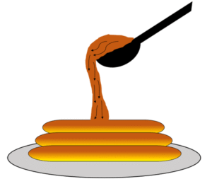
Figure 5: Honey flowing smoothly from a spoon as an everyday example of laminar flow
Example of turbulent flow
Turbulent flow surrounds us in everyday life and dominates most fluid flow situations we encounter. For instance, the white, frothy water in rivers and streams demonstrates classic turbulent flow characteristics with visible eddies and vortices swirling in unpredictable patterns. When you observe smoke rising from a cigarette, you’ll notice it initially rises in a straight, laminar flow pattern. However, it quickly transitions to turbulent flow as it moves upward, creating the familiar swirling patterns we associate with smoke. This visual example perfectly illustrates the laminar to turbulent flow transition that occurs as the Reynolds number increases with distance from the source.
Fast-flowing water from a fully opened faucet exemplifies turbulent flow. In addition to the visible turbulence, this flow regime creates the characteristic rushing sound we associate with flowing water. This noise results from pressure fluctuations within the chaotic turbulent flow. In aerospace applications, the air flow over aircraft wings typically transitions from laminar flow near the leading edge to turbulent flow as it moves toward the trailing edge. Furthermore, understanding and controlling this transition is crucial for optimizing aerodynamic performance. In fact, engineers sometimes use special surface treatments or designs to delay the onset of turbulence and reduce drag.

Figure 6: Smoke rising from a cigarette – transition from laminar to turbulent flow regime
Laminar flow Vs turbulent flow Reynolds number
The Reynolds number serves as the key parameter that distinguishes between laminar and turbulent flow regimes. This dimensionless quantity represents the ratio of inertial forces to viscous forces within a fluid. Moreover, it’s calculated using the formula, where ρ is fluid density, v is velocity, D is characteristic length, and μ is dynamic viscosity.
![\[ Re=\frac{pVL}{u} \]](https://cfdland.com/wp-content/ql-cache/quicklatex.com-935d1a769d4487db1d8a1cbe682003d1_l3.png "Rendered by QuickLaTeX.com")
For pipe flows, the difference between laminar and turbulent flow becomes apparent at specific Reynolds number thresholds. Generally, flow remains laminar when the Reynolds number is below approximately 2,300. Additionally, between 2,300 and 4,000, the flow enters a transitional regime where it shows characteristics of both laminar and turbulent flow. Furthermore, when the Reynolds number exceeds 4,000, the flow becomes fully turbulent. The laminar to turbulent flow transition doesn’t occur at a single point but rather over a range of Reynolds numbers. In fact, this transition can be affected by factors like surface roughness, flow disturbances, and fluid properties. Consequently, predicting the exact transition point requires consideration of these additional variables beyond just the Reynolds number. Understanding the relationship between Reynolds number and flow regimes is crucial in engineering applications. You can read more about Reynolds number in below blog.

Figure 7: What is reynolds number?
Difference between laminar, turbulent, and transitional flow
The difference between laminar and turbulent flow extends beyond their basic definitions. Laminar flow is characterized by fluid particles moving in parallel layers with minimal mixing between them. On the other hand, turbulent flow features chaotic motion with extensive mixing and fluctuating properties. In addition to these two main flow regimes, transitional flow represents an intermediate state where both laminar and turbulent flow characteristics coexist. During this transitional phase, portions of the flow may exhibit laminar flow behaviors while others show signs of emerging turbulence. As a result, transitional flow can be particularly challenging to predict and model accurately.
The difference between laminar and turbulent flow also becomes evident in their energy characteristics. Laminar flow generally has lower energy dissipation rates since fluid layers slide past each other with minimal interaction. Conversely, turbulent flow dissipates energy more rapidly due to the work done by eddies and vortices against viscous forces. Furthermore, this higher energy dissipation in turbulent flow typically results in greater pressure drops in practical applications. Flow visualization techniques can clearly reveal the difference between laminar and turbulent flow regimes. In laminar flow, dye injected into the fluid will follow straight, parallel streamlines with minimal dispersion. However, in turbulent flow, the same dye would quickly disperse throughout the fluid as it’s carried by chaotic eddies and mixing currents. Indeed, these visual distinctions provide engineers with practical methods to identify flow regimes in experimental settings.
What is Rayleigh number?
While the Reynolds number governs the transition from laminar to turbulent flow in forced convection scenarios, the Rayleigh number plays a similar role in natural convection processes. The Rayleigh number represents the relationship between buoyancy forces and viscous forces in a fluid, determining whether heat transfer occurs primarily by conduction or convection. The Rayleigh number directly influences whether natural convection flows will be laminar or turbulent. Additionally, low Rayleigh numbers typically result in laminar flow patterns, while high values lead to turbulent flow. Furthermore, this dimensionless parameter helps engineers predict heat transfer rates in systems where flow is driven by density differences rather than external pressure.
![\[ Ra=\frac{gß(T_s-T∞)x^3}{Va} \]](https://cfdland.com/wp-content/ql-cache/quicklatex.com-87ed88ae18b6aca459b91f39ca987e78_l3.png "Rendered by QuickLaTeX.com")
Where g [m.s-2] is the acceleration due to gravity, β [1.K-1] is the thermal expansion coefficient of the fluid, x [m] is the characteristic length scale, α [m2.s] is the thermal diffusivity of the fluid, ν [m2.s] is the kinematic viscosity of the fluid, TS [K] is the surface temperature and T∞ [K] is fluid temperature.
Natural convection becomes particularly important in many practical applications such as passive cooling systems, weather patterns, and oceanic currents. Moreover, understanding the relationship between Rayleigh number and flow regimes allows engineers to design more efficient heating and cooling systems. In fact, optimizing these systems often involves manipulating conditions to achieve either laminar or turbulent flow, depending on the desired heat transfer characteristics.
The Rayleigh number complements the Reynolds number in providing a complete picture of flow regime determination. Consequently, both parameters are essential tools in fluid dynamics analysis, especially for computational fluid dynamics (CFD) simulations that need to accurately model both forced and natural convection processes.

Figure 8. Free convection boundary layer transition on a vertical plate, from “Fundamentals of heat and mass transfer” by Frank P. Incropera et al.
In natural convection, the flow regime is determined by the Rayleigh number, not the Reynolds number. Figure 8 shows natural convection flow on a vertical plane. As can be seen, the flow regime changes at Ra = 109, which is called the critical Rayleigh number. Natural convection currents are created due to the temperature difference in the fluid, which causes a density difference and the resulting buoyancy force.
The flow regime in ANSYS Fluent
ANSYS Fluent, a leading computational fluid dynamics (CFD) software, offers sophisticated tools for modeling both laminar and turbulent flow regimes. When setting up a simulation in Fluent, engineers must first specify whether to use a laminar flow model or one of several turbulence models based on the expected flow characteristics. For laminar flow simulations, Fluent directly solves the Navier-Stokes equations without additional turbulence modeling. This approach works well for flows with low Reynolds numbers where the laminar flow characteristics dominate. Additionally, these simulations typically require less computational resources since they don’t need to resolve small-scale turbulent structures.
When modeling turbulent flow, Fluent offers various approaches including RANS (Reynolds-Averaged Navier-Stokes), LES (Large Eddy Simulation), and DES (Detached Eddy Simulation) methods. Furthermore, each approach makes different trade-offs between computational cost and accuracy in capturing turbulent flow characteristics. As a matter of fact, selecting the appropriate turbulence model requires understanding both the physics of the problem and the limitations of each modeling approach.
In Ansys Fluent, the user determines the flow regime by calculating the Reynolds number (or Rayleigh number in case of natural convection) outside the software. Based on this calculation, it is determined whether the flow simulation is laminar or turbulent.
There are several methods in Fluent to simulate turbulent flow. Each of them has its advantages and disadvantages and is suitable for specific applications.
Under the title of “Viscous Models” in the software, all the simulation methods for the fluid flow regime available in the software are:
- Inviscid: In this model, it is assumed that fluid has no viscosity.
- Laminar: There is just one model for viscous laminar flows and it solves ordinary Navier-Stokes equation. The following models are for simulating turbulent flow
- Spalart-Allmaras: It is a Reynolds-Averaged Navier-Stokes (RANS) model, suitable for aerodynamics applications.
- k-epsilon: It is a Reynolds-Averaged Navier-Stokes (RANS) model, suitable for general-purpose turbulence modeling in various applications.
- k-omega: It is a Reynolds-Averaged Navier-Stokes (RANS) model, suitable for modeling near-wall and low-Reynolds number turbulence.
- Transition k-kl-omega: It is a Reynolds-Averaged Navier-Stokes (RANS) model, suitable for modeling transitional flows from laminar to turbulent.
- Transition SST: This model is a combination of the k-epsilon and k-omega turbulence models.
- Reynolds Stress it is a RANS model suitable for simulating highly anisotropic turbulent flows.
- Scale-Adaptive simulation: A hybrid RANS-LES model suitable for resolving different turbulent scales.
- Detached Eddy Simulation: A hybrid RANS-LES model suitable for resolving eddies near walls.
- Large Eddy Simulation (LES): A method resolving large turbulent structures, suitable for high-resolution simulations. It is not a RANS model.
The details of each viscous model can be adjusted in the software. For example, for the k-epsilon model, there are three modes: standard, RNG, and realizable.

Figure 9. Viscous models, ANSYS Fluent
Conclusion
Understanding the difference between laminar and turbulent flow is fundamental in fluid dynamics and has far-reaching implications across numerous fields of science and engineering. The transition from laminar to turbulent flow, governed primarily by the Reynolds number, represents one of the most important phenomena in fluid behavior. Laminar flow characteristics include orderly, parallel fluid layers with predictable velocity profiles and minimal mixing. In contrast, turbulent flow characteristics involve chaotic motion with extensive mixing, fluctuating properties, and complex eddy structures. Additionally, transitional flow represents the intermediate stage where both laminar and turbulent flow features coexist.
The Reynolds number serves as the key parameter for distinguishing between these flow regimes, with low values indicating laminar flow and high values pointing to turbulent flow. Furthermore, other parameters like the Rayleigh number help characterize flows driven by buoyancy forces rather than external pressure differentials.
Modern computational tools like ANSYS Fluent enable engineers to simulate and analyze both laminar and turbulent flow scenarios with increasing accuracy. As a result, these simulations provide valuable insights for designing everything from aircraft wings to blood pumps. Indeed, the continuous advancement in our understanding of flow regimes and our ability to model them computationally promises to drive innovation across numerous industries for years to come.
Related Blogs
Explore the various categories and models of turbulent flow that engineers use to simulate complex fluid behavior beyond the basic laminar vs turbulent flow distinction.
Discover an advanced computational approach specifically designed to capture the complex eddy structures and chaotic behavior of turbulent flow regimes.
Learn how temperature differences create buoyancy-driven flows that can exhibit both laminar and turbulent characteristics similar to those governed by the Reynolds number.
Understand the fundamental principles behind simulating and analyzing flow regimes using computational methods like those in ANSYS Fluent mentioned in our article.