
In real-life engineering, chaotic fluid motion is everywhere. From the aerodynamics of vehicles to the thermal mixing in industrial heat exchangers, engineers should account for highly unpredictable flow behaviors. However, despite decades of research, no general analytical solution exists to calculate these complex flows directly!
Because computing every microscopic velocity fluctuation requires impossible computational power, computational fluid dynamics (CFD) relies on turbulence models. These mathematical approximations predict the statistical and average behavior of the fluid. Choosing the correct model is the only way a solver can accurately estimate critical design parameters like pressure drop, thermal dissipation, and wall shear stress.
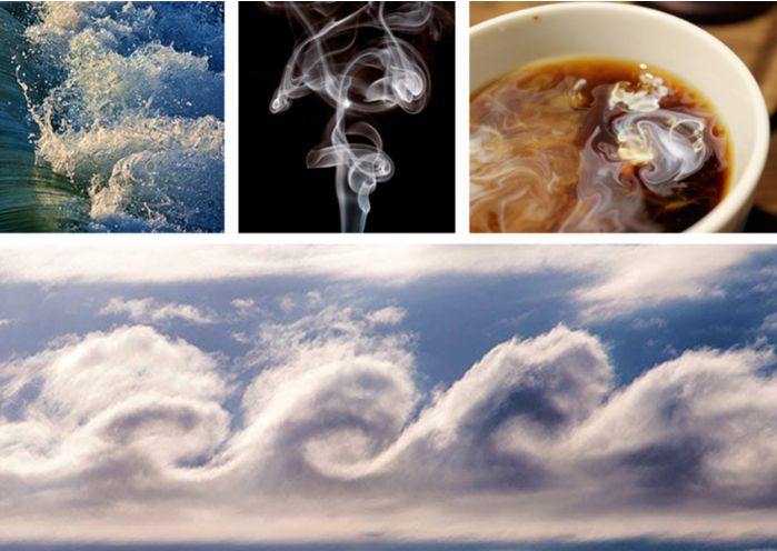
Figure 1: Examples of turbulent dynamics in real-life and engineering applications (credits: Paul Chartier)
Note: If you are unsure whether your system operates in a stable or chaotic regime, first review our physical guide on the difference between laminar and turbulent flow before configuring your CFD setup.
Why Turbulent Flow Cannot Be Solved Directly
To understand why we need a turbulence model, we have to look at the governing equations of fluid dynamics: the Navier-Stokes equations. When a fluid moves in a smooth, predictable manner, CFD solvers compute these equations directly. However, as we know from the characteristics of turbulent flow, chaotic motion introduces rapid, random fluctuations in velocity and pressure across space and time.
Currently, resolving every microscopic instantaneous fluctuation requires computing power that is impossible for standard industrial design. Instead of calculating every tiny eddy, engineers need to know the average behavior of the fluid. In 1895, Osborne Reynolds proposed a mathematical solution: splitting the flow properties into a mean (average) component and a fluctuating component.
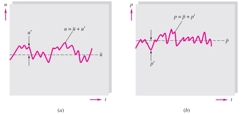
Figure 2: Definition of mean and fluctuating turbulent variables: (a) velocity; (b) pressure)
This mathematical approach is called Reynolds decomposition. For any variable, such as velocity (u), we divide it into a time-averaged value (uˉ) and a fluctuating part (u′):
u' = u - \bar{u}
By definition, the time average of the fluctuation itself is zero (u′ˉ=0). However, when we substitute this split variable back into the Navier-Stokes equations and time-average the entire equation, something important happens. The non-linear acceleration terms produce mean products of the fluctuating velocities, such as u′v′‾. The average of these multiplied fluctuations is not zero.
When multiplied by the fluid density (ρ), these new terms (−ρu′v′‾) act mathematically like additional internal friction on the fluid. We call them the Reynolds stresses.
This creates a critical mathematical barrier known as the turbulence closure problem. We now have extra unknown variables (the Reynolds stresses) in our equations, meaning we have more unknowns than we have equations. We cannot close the mathematical loop.
To solve the Reynolds-Averaged Navier-Stokes (RANS) equations, we must introduce a new mathematical approximation to calculate these unknown stresses without computing the chaotic eddies directly. (For a deep look at how the energy of these fluctuations is tracked mathematically, review the transport equations for turbulent kinetic energy and dissipation rate).
The Eddy Viscosity Concept
In the previous section, we saw how Reynolds time-averaging creates the turbulence closure problem. We are left with unknown Reynolds stresses that we must calculate to complete our simulation.
In 1877, Joseph Boussinesq proposed a brilliant simplification. He suggested that the chaotic mixing caused by turbulent eddies acts just like the fluid’s natural internal friction, only on a much larger scale. Instead of trying to compute the complex Reynolds stresses directly, the Boussinesq hypothesis replaces them with a single new variable: turbulent viscosity (also known as eddy viscosity).
While a fluid’s molecular viscosity is a fixed physical property (like honey being thicker than water), eddy viscosity is a dynamic property of the flow itself. A CFD solver calculates this extra viscosity and adds it to the natural viscosity of the fluid. This mathematical trick closes the equations. Almost all standard turbulence models in CFD are simply different mathematical recipes for calculating this single turbulent viscosity value.
How Turbulence Models Are Classified
With the mathematical foundation established, we classify a CFD turbulence model based on one simple question: how much of the turbulent motion do we resolve directly on the mesh, and how much do we model using equations?
This creates a spectrum of computational cost and accuracy.
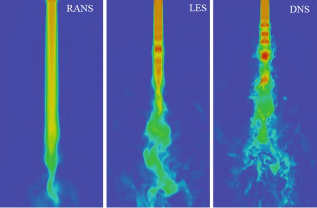
Figure 3- Turbulence models in CFD and their accuracy in flow simulation
- Direct Numerical Simulation (DNS): This approach resolves all turbulent fluctuations down to the smallest microscopic scale. It requires extreme computational power and is primarily reserved for academic research.
- Large Eddy Simulation (LES): This method sits in the middle of the spectrum. It computes the large eddies directly and only models the small ones. If you need to capture highly unsteady flow separation, read our complete guide on how large eddy simulation resolves the larger eddies.
- Reynolds-Averaged Navier-Stokes (RANS): This approach models all turbulence using time-averaging and eddy viscosity. Because of its low computational cost, RANS is the highly efficient industry standard for most engineering design work.
- Hybrid Models (DES/SAS): These methods combine RANS near the walls with LES in the mainstream. For advanced aerodynamic cases, read our guide on hybrid RANS-LES approaches such as DES.
Because RANS methods offer the best balance of acceptable accuracy and low computational cost, they remain the standard choice for the vast majority of industrial CFD simulations.
The RANS Model Family
Because computing every chaotic fluctuation directly is too expensive, the Reynolds-Averaged Navier-Stokes (RANS) approach is the most common choice for industrial engineering. As we discussed, these models rely entirely on the Boussinesq hypothesis. Their only job is to calculate the turbulent viscosity.
How do they calculate it? They solve additional transport equations alongside the momentum and continuity equations. We classify these RANS turbulence models by the number of extra equations they add to the solver. Let us look at the three foundational models.
1. The Spalart-Allmaras Model (1-Equation)
This model adds only 1 extra equation to the CFD solver. Instead of calculating intermediate turbulent properties, it calculates the kinematic eddy viscosity directly.
- Convenient for: External aerodynamics, transonic flows over airfoils, and general aerospace applications. It requires low computational power, is highly stable, and converges easily.
- Limitations: Because it is so simple, it struggles to predict complex shear flows, heavy flow separation, and decaying turbulence.
2. The Standard k-epsilon Model (2-Equation)
The k-epsilon turbulence model is the most famous two-equation model in CFD history. It solves two extra transport equations: one for turbulent kinetic energy (k) and one for the rate of dissipation (ϵ).
- Convenient for: General-purpose industrial flows, external flows far away from walls, and complex geometries. It requires relatively low memory and offers excellent convergence.
- Limitations: It assumes the flow is fully turbulent. Therefore, it performs poorly close to no-slip walls, in flows with strong curvature, and under adverse pressure gradients (such as expanding pipes).
3. The Standard k-omega Model (2-Equation)
Instead of calculating the dissipation rate (ϵ), the k-omega model solves for the specific dissipation rate (ω). This change in the mathematics completely alters how the model behaves near a solid boundary.
- Convenient for: Internal flows, resolving the boundary layer close to the walls, and predicting flow separation under adverse pressure gradients.
- Limitations: The standard version of this model is highly sensitive to the initial free-stream conditions at the inlet. If you guess the wrong inlet values, the simulation will produce inaccurate results.
To solve the specific weaknesses of standard k−ϵ and standard k−ω, researchers combined them into hybrid models. In the next section, we will compare the two most important models used in modern CFD.
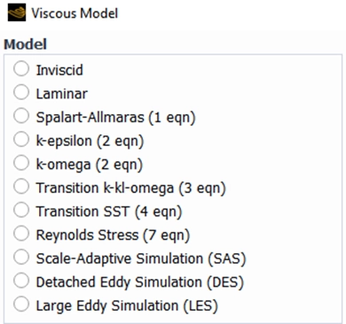
Figure 4: Turbulence Models in the Viscous Model Setup of ANSYS Fluent
k-epsilon vs k-omega SST
For decades, engineers faced a difficult choice when selecting a CFD turbulence model. As we learned in the previous section, the standard k−ϵ model is highly stable and performs excellently in the free stream (far from walls), but it fails to accurately predict flow separation near solid boundaries. Conversely, the standard k−ω model resolves the near-wall boundary layer beautifully, but it is highly unstable and sensitive to the inlet conditions in the free stream.
To solve this dilemma, F.R. Menter developed the k−ω SST (Shear Stress Transport) model.
The SST formulation is a hybrid approach. It uses a mathematical blending function to combine the best features of both models:
- Near the solid walls: The blending function activates the k−ω formulation to accurately capture the boundary layer and flow separation.
- In the free stream: The blending function smoothly switches to the k−ϵ formulation, avoiding the free-stream sensitivity problems of standard k−ω.
Additionally, the SST formulation limits the principal turbulent shear stress to prevent the model from over-predicting turbulent viscosity in areas with high pressure gradients.
The Verdict: Today, the k−ω SST model is considered the industry standard for most aerospace, automotive, and complex industrial simulations. Unless you have a specific reason to use a simpler model, SST offers the best balance of accuracy and reliability for flows with adverse pressure gradients and separation. The table below summarizes the differences from different aspects:
| Feature | k-epsilon (Standard) | k-omega SST |
|---|---|---|
| Near-Wall Treatment | Requires empirical wall functions | Resolves the boundary layer directly |
| Separated Flow | Over-predicts eddy viscosity; delays separation | Superior prediction of adverse pressure gradients |
| Free-Stream Sensitivity | Highly robust; insensitive to free-stream values | Blending function protects it from instability |
| Complexity & Mesh | Faster convergence, allows a coarser mesh | Complex; requires a very fine mesh near walls |
Note: If our simulation goal involves predicting the precise point of separation or complex recirculating flow patterns, k-omega SST is the necessary choice. However, we must be prepared to build a much finer mesh near the walls. Using k-omega SST correctly requires specific near-wall mesh sizing (specifically, a y+≈1). As a result, for high-speed, attached flow scenarios where far-field convergence is our main priority, k-epsilon provides a highly efficient solution.
Turbulence Models in the ANSYS Fluent Viscous Model Panel
When we open ANSYS Fluent to configure a CFD simulation, we should define the mathematical behavior of the fluid. We do this inside the Viscous Model setup window. This panel contains all the primary CFD turbulence models we have discussed, plus a few advanced options. Here is a practical breakdown of what each selection means for your simulation.
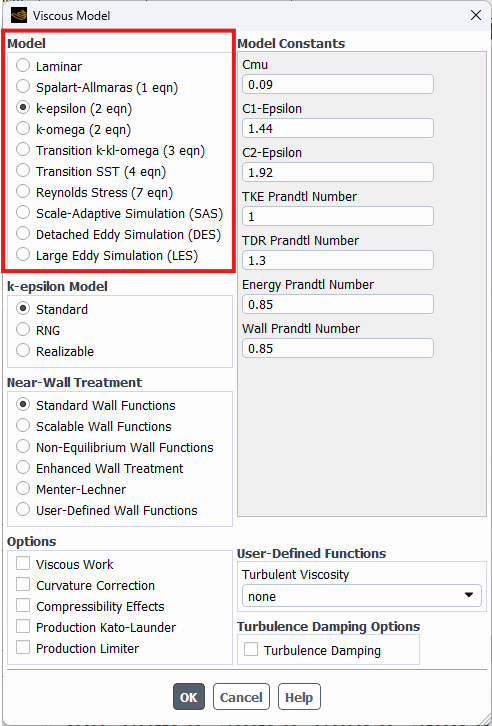
Figure 5: Turbulence Models in the Viscous Model Setup of ANSYS Fluent)
- Inviscid: This assumes the fluid has absolutely zero viscosity. We use this only for highly simplified, ideal flow theories where friction does not matter.
- Laminar: This models smooth, orderly flow without any chaotic mixing or eddies. It is strictly for low Reynolds number flows.
- Spalart-Allmaras (1 Equation): As discussed, this is a fast, single-equation model designed primarily for aerospace and external aerodynamic boundary layers.
- k-epsilon (2 Equations): The industry standard for general purposes. Selecting this opens up sub-variants, including the Standard, RNG, and Realizable formulations, depending on your specific internal flow needs.
- k-omega (2 Equations): The required choice for resolving boundary layers and adverse pressure gradients. Selecting this allows you to activate the crucial SST (Shear Stress Transport) hybrid formulation.
- Transition Models (3 & 4 Equations): Options like Transition k-kl-omega and Transition SST are specialized models. We use them specifically when we need to capture the exact physical point where a boundary layer changes from laminar to turbulent.
- Reynolds Stress Model (RSM) (7 Equations): Instead of using the Boussinesq (eddy viscosity) hypothesis, this highly complex model solves separate transport equations for every individual directional stress. We reserve it for highly anisotropic flows, such as strong cyclones or swirling combustion chambers.
- Large Eddy Simulation (LES): This resolves the large turbulent structures directly while modeling the small ones. Because it requires specific mesh and time-step sizing, you can follow our complete guide on LES implementation in ANSYS Fluent.
- Hybrid Models (DES & SAS): These methods (like Detached Eddy Simulation) combine RANS near the walls with LES in the free stream.
How to Choose a Turbulence Model
Selecting the most suitable CFD turbulence model can feel overwhelming for beginners. As a general rule, there is always a trade-off between computational simplicity and the richness of the flow information obtained. To make this decision easier, we recommend following a clear, four-step process to ensure your simulation is both accurate and computationally efficient.
Step 1: Define Your Goal
First, ask yourself what data you actually need.
- If you primarily need the average flow behavior, drag forces, or general pressure drops, RANS is the correct and most efficient choice.
- If your project requires capturing time-varying phenomena, aeroacoustics, or highly dynamic vortex shedding, you will need to invest the heavy computational resources required for LES or DES.
Step 2: Match the RANS Model to the Physics
If you choose the RANS family (like 90% of industrial simulations), scrutinize the physical incident and select the model that fits the flow behavior:
- Is it external aerodynamics without severe separation? (e.g., an airplane wing at cruising altitude). Start with the Spalart-Allmaras model. It is fast and highly stable.
- Is it a general internal flow or complex geometry? (e.g., flow through a large HVAC room or a simple pipe). The k−ϵ model (especially the Realizable variant) is highly robust and forgives coarse meshes.
- Does it involve adverse pressure gradients, heat transfer, or severe flow separation? (e.g., diffusers or stalled airfoils). You must use the k−ω SST model. Just remember that it requires a very fine mesh near the walls.
Step 3: Check the Literature
Before setting up your CFD solver, always research existing literature. Look for experimental validation studies or academic papers that feature geometries similar to yours. If a published paper proves that a specific model performs best for a certain type of hydrocyclone or wind turbine, use their findings as your starting point.
Step 4: Validate and Compare
If the literature is poor or your geometry is entirely unique, you should run a sensitivity study. Try running your simulation with two different models (for example, run it once with k−ϵ and once with k−ω SST) and compare the results against experimental data. Validation is the only way to guarantee your mathematical approximation matches physical reality.
Common Turbulence Modeling Mistakes
Even with the most powerful CFD solvers, a poor setup will always produce inaccurate results. When working with turbulence models, engineers frequently make these four critical errors:
- Ignoring Mesh Requirements: As we discussed, advanced models like k−ω SST require a very fine computational mesh near the solid walls. Applying a highly complex model to a coarse mesh will often yield worse results than using a simple model. Always verify your grid resolution!
- Using Steady-State for Unsteady Flows: If your flow features heavy vortex shedding (such as air flowing over a blunt cylinder), a steady-state RANS solver will struggle to converge. You must switch to a transient (time-dependent) formulation.
- Guessing Inlet Conditions Blindly: Leaving the Turbulence Intensity at the solver’s default value for every single simulation is a major mistake. Always calculate or estimate the physical mixing rate entering your specific system.
- Skipping Experimental Validation: A computational formulation is merely a mathematical approximation. Whenever possible, always compare your turbulent flow results with real-world experimental data or established literature to ensure your chosen approach is accurate.
Conclusion
Understanding turbulence remains one of the greatest challenges in classical physics. However, by learning how to classify and apply the correct CFD turbulence models, you can accurately predict complex fluid behavior in your engineering projects. Whether you need the rapid efficiency of RANS for an industrial pipe network or the high fidelity of Large Eddy Simulation (LES) for aerodynamic research, selecting the right mathematical approach is the foundation of a successful simulation. Always start simple, build a high-quality mesh, and match your model to the physical flow characteristics.
At CFDLAND, we are dedicated to helping engineers and researchers learn turbulence modeling in CFD. If you are ready to put this theory into practice, we have the resources to support you:
- Explore our CFDSHOP for a wide range of prepared simulation files and a verified turbulent flow ANSYS Fluent examples.
- If you need personalized assistance with your setup, Visit our Order CFD Project for custom solutions tailored to your specific analysis.