Turbulent Kinetic Energy (k) and Dissipation Rate (ε)

In a turbulent flow, the fluid does not move in smooth, simple layers. It contains small and large eddies. These eddies alter the velocity, pressure, mixing, and heat transfer in the domain. In ANSYS Fluent, two important values help the solver model this behavior: turbulent kinetic energy (k) and turbulence dissipation rate (ε).

In simple terms, k shows how strong the turbulence is, and ε shows how fast this turbulent energy is lost.

These two values are fundamental in the k-epsilon turbulence model. Fluent uses them to calculate turbulent viscosity, which heavily impacts engineering results. It can change the pressure drop in a pipe, wall shear stress near a surface, outlet temperature in a heat transfer case, or mixing quality in a jet flow. Therefore, incorrect values of k and ε can produce a result that looks converged but is physically wrong.

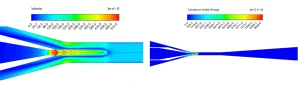
Figure 1: Turbulent flow in ANSYS Fluent. Velocity and turbulence kinetic energy contours help show where eddies and strong mixing appear in the domain.

Engineers often encounter these terms in boundary conditions, solver settings, residuals, and post-processing. For example, when setting an inlet, ANSYS Fluent may ask for turbulence intensity, hydraulic diameter, length scale, or direct values of k and ε. These inputs define the initial turbulence field at the inlet.

The same principle applies after the simulation. A good CFD result should not be judged solely by residuals. You must also analyze velocity, turbulence kinetic energy, dissipation rate, and turbulent viscosity contours. High turbulence should appear in logical places, such as wakes, jets, shear layers, recirculation zones, and near-wall regions.

This guide explains these variables practically, covering their meaning, their role in the model, inlet calculation methods, common warnings, and contour interpretation.

What Are Turbulent Kinetic Energy and Dissipation Rate?

In a turbulent flow, the velocity at one point is not constant. It changes constantly with time and direction. These changes are called velocity fluctuations.

These fluctuations create eddies, which drive mixing, momentum transfer, heat transfer, and energy loss. In the k-epsilon model, two main variables describe this process:

• Turbulent kinetic energy (k): Shows how strong the turbulent motion is.
• Turbulence dissipation rate (ε): Shows how fast this turbulent energy is destroyed.

This is why k and ε are not just mathematical values; they are vital engineering signals indicating whether your flow field is physical.

Turbulent Kinetic Energy (k): The Strength of Turbulence

Turbulent kinetic energy represents the kinetic energy of velocity fluctuations. It indicates the energy level of the turbulent eddies.

For a three-dimensional flow, k is defined as:

k = \frac{1}{2} (u’^2 + v’^2 + w’^2)

Here, u’, v’, and w’ are velocity fluctuations in three directions. The unit of k is: m²/s² (or J/kg).

A high value of k means strong turbulent motion. You often see high turbulence kinetic energy in jets, wakes, mixing layers, recirculation zones, and separated flows. For instance, the wake behind a cylinder possesses high k due to strong unsteady eddies. However, high k is not automatically good or bad. High k in a wake is physical, but high k in a calm inlet region usually indicates an incorrect boundary condition.

Turbulence Dissipation Rate (ε): The Loss of Turbulent Energy

The turbulent dissipation rate (ε) shows how quickly turbulent kinetic energy changes into internal energy (heat) due to fluid viscosity.

Large eddies extract energy from the mean flow and break into smaller eddies. At the smallest scales, viscosity destroys this turbulent energy. This final loss process is called dissipation.

The unit of ε is: m²/s³ (or W/kg).

A high ε value means turbulent energy is lost quickly, frequently occurring near walls, in strong shear layers, and in high-strain regions. A low ε value means the energy degrades slowly. If ε becomes too low while k is high, ANSYS Fluent may calculate an unrealistically large turbulent viscosity.

Energy Cascade: The Physical Link Between k and ε

In turbulent flow, energy moves through many eddy sizes in a process called the energy cascade.

First, the mean flow gives energy to large eddies created by the inlet flow, wall shear, or obstacles. They contain most of the turbulent kinetic energy. These large eddies become unstable and break into smaller ones. In this middle range, energy transfers from one scale to the next without being lost.

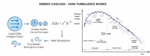
Figure 2: Energy Cascade, The Physical Link Between k and ϵ

At the smallest eddy scales, velocity gradients become extreme. Here, fluid viscosity converts turbulent kinetic energy into heat. This final step is viscous dissipation.

This energy path can be shown as:

Therefore, k relates to the energy stored in the eddies, while ε relates to the final destruction of that energy. The energy cascade explains why they must be checked together. In CFD, resolving every tiny eddy is computationally impossible, so we model the cascade’s effects using these two variables.

How k and ε Work Inside the k-Epsilon Model

The k-epsilon model is a two-equation Reynolds-Averaged Navier-Stokes (RANS) model. It does not resolve small eddies directly. Instead, it solves one transport equation for k and one for ε.

These variables allow the solver to estimate a turbulent velocity scale and a turbulent length scale:

• Turbulent time scale: τ = k / ε
• Turbulent length scale: l = (k^(3/2)) / ε

Most importantly, Fluent uses k and ε to calculate the turbulent viscosity (μt), which dictates mixing, pressure loss, and wall shear stress:

\mu_t = \rho C_\mu \frac{k^2}{\epsilon}

Here, ρ is fluid density, and Cμ is a model constant (usually 0.09).

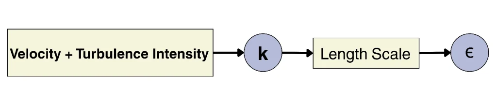
Figure 3: Role of k and ϵ in the k-epsilon model. Fluent uses these two values to calculate turbulent viscosity and predict turbulent flow behavior.

If k is too high or ε is too low, the calculated turbulent viscosity becomes massive. The flow may appear smooth and converged, but the physics will be completely incorrect. This is why checking contours is mandatory.

The standard transport equations for these variables include production terms (where mean velocity gradients generate turbulence) and destruction terms. For example, high k production occurs when the mean flow has strong velocity gradients, which is why boundary layers and wakes show high turbulence.

These variables are equally critical when simulating complex multiphase systems. Properly assigning them is a core requirement when setting up Turbulence Modeling in Eulerian Multiphase Flows.

Figure 4: Turbulence Modeling in Eulerian Multiphase Flows article in CFDLAND

Difference Between k and ε

Table 1 summarizes the practical differences when analyzing results.

Item	Turbulent Kinetic Energy (k)	Turbulence Dissipation Rate (ε)
Meaning	Strength of turbulence	Rate of turbulent energy loss
Physical Role	Shows energy in eddies	Shows energy destruction by viscosity
Fluent Role	Defines turbulent motion	Defines turbulent length/time scale
Unit	m²/s²	m²/s³
High-value Zones	Jets, wakes, shear layers, mixing	Near walls, high-strain zones
Effect on μt	Higher k increases μt	Higher ε decreases μt

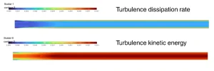
Figure 5: Turbulence kinetic energy and turbulence dissipation rate contours in ANSYS Fluent. The k contour shows strong turbulent motion, while the ϵ contour shows where turbulent energy is lost quickly.

Which Turbulence Specification Method Should Be Used?

The standard k-epsilon family includes Standard, RNG, and Realizable models. While Standard is highly stable, Realizable handles rotation and separation better. Choosing the right one is essential for any turbulence CFD simulation to ensure accurate wake and pressure field predictions.

The user should choose the turbulence model based on the flow physics. The goal is not only convergence. The goal is a physical turbulence field. For rotating flow, for example, different models can predict different wake and pressure fields. A useful practical case is the Effect of Different Turbulence Models on Savonius CFD Simulation, where k-epsilon-based results can be compared with other turbulence models.

Figure 6: Savonius turbine CFD simulation with different turbulence models. This example shows why model choice can change the predicted flow field.

Fluent gives different ways to define inlet turbulence. The user should choose the method based on the available data. Direct input of k and epsilon is good only when the user has trusted values from an experiment, a previous simulation, or a clear calculation.

Table 2: Common inlet turbulence methods in ANSYS Fluent.

Fluent Inlet Method	When It Is Useful	Simple Note
Intensity and Hydraulic Diameter	Pipe, duct, and channel flow	Good for many internal flow cases
Intensity and Length Scale	Jet flow, external flow, open domains	Useful when the main turbulence size is known
Intensity and Viscosity Ratio	General cases with limited data	Simple, but less direct
k and ϵ	Cases with known turbulence data	Use only with trusted values
k and Turbulent Viscosity Ratio	Some advanced setup cases	Needs care and checking

For pipe and duct flow, Intensity and Hydraulic Diameter is often the safest first choice. For jet flow and open domains, Intensity and Length Scale can be more suitable. If the user enters direct values of k and ϵ, the values should be checked with contours after the solution.

It is better to change one input at a time. For example, do not change inlet velocity, turbulence intensity, mesh, and wall treatment all together. If the result changes, the user will not know the main reason. A step-by-step setup is slower, but it gives a more reliable CFD result.

How to Calculate k and ε for Inlet Boundary Conditions

The inlet boundary condition is your first interaction with k and ε. The solver needs a realistic initial turbulence estimate before it can calculate downstream mixing and separation.

If the inlet turbulence is too high, the domain becomes excessively diffusive. If it is too low, mixing will be improperly weak. This is a common issue when setting up advanced fluid mechanics CFD simulation cases.

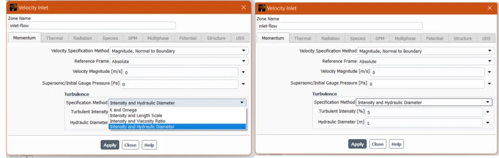
Figure 9: Inlet turbulence settings in ANSYS Fluent. The selected method gives Fluent the first estimate of k and ϵ at the inlet.

Because direct experimental values of k and ε are rarely known, engineers typically use Turbulence Intensity, Hydraulic Diameter, or Turbulent Length Scale.

1. Calculate k from Turbulence Intensity

k = \frac{3}{2} (U \cdot I)^2

Where U is the mean inlet velocity (m/s) and I is the turbulence intensity (entered as a decimal, e.g., 0.05 for 5%).

For internal flows, turbulence intensity can also be estimated from the Reynolds number:

This is only an estimate. It is useful when there is no measured turbulence data.

2. Calculate ε from Length Scale

\epsilon = C_\mu^{3/4} \frac{k^{3/2}}{l}

For internal duct flows, the length scale (l) is typically estimated as l = 0.07 * Dh, where Dh is the hydraulic diameter. C_μ is usually 0.09. 

For many internal flows, the length scale can be estimated as:

l = 0.07 D_h

For instance, assume air enters a duct with:

• Mean velocity: U = 10 m/s
• Turbulence intensity: I = 5% = 0.05
• Hydraulic diameter: Dh = 0.1 m

First, calculate k:

k = 1.5 \cdot (10 \cdot 0.05)^2 = 1.5 \cdot (0.25) = \textbf{0.375 m}^2/\textbf{s}^2

Next, calculate the length scale:

l = 0.07 \cdot 0.1 = \textbf{0.007 m}

Finally, calculate ε (assuming Cμ = 0.09):

\epsilon = (0.09^{0.75} \cdot 0.375^{1.5}) / 0.007 = (0.1643 \cdot 0.2296) / 0.007 = \textbf{5.39 m}^2/\textbf{s}^3

These physical estimates stabilize the solver instantly compared to guessing random inputs.

Figure 10: Simple workflow for calculating inlet k and ϵ. The user can estimate turbulence kinetic energy from velocity and turbulence intensity, then calculate epsilon from length scale.

Practical Checks Before Running the Solver

Before clicking “Calculate”, run through this checklist to prevent divergence:

1. Check Intensity Formats: Ensure turbulence intensity is entered correctly (some panels require percentages, some require decimals).
2. Verify Hydraulic Diameter: Confirm the Dh matches your actual inlet geometry, not the default 1m.
3. Inspect the Mesh: Poorly generated cells at the inlet will instantly multiply initial k values into numerical errors.
4. Confirm y+ Strategy: Ensure your first cell height matches your chosen wall treatment.
5. Review Backflow Settings: Ensure the pressure outlet has realistic backflow turbulence intensity (typically 5%) to prevent errors if reverse flow occurs.

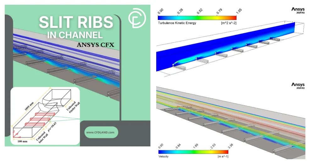
Figure 11: Turbulence kinetic energy contour after inlet setup. The contour helps check if the inlet turbulence level is realistic.

Common Fluent Warnings and Errors

A simulation can converge while generating physically incorrect turbulence.

• “turbulent viscosity ratio limited”

This warning means ANSYS Fluent calculated an exceptionally high turbulent viscosity compared to molecular viscosity. Because μt depends on k²/ε, this happens when k is too high or ε is too low. If it occurs only during the first few iterations, it is usually harmless. If it persists, you must check your mesh quality or inlet parameters.

• Divergence in k or ε Equations

If the k or ε residuals rise sharply, the solver cannot stabilize the turbulence transport equations. Change one setting at a time: review inlet values, verify outlet backflow, and check the wall region.

Fluent Problem	Possible Cause	First Check
Turbulent viscosity ratio limited	High k or low ε	Check inlet intensity and length scale
k residual rises fast	Inlet turbulence too high	Reduce turbulence intensity
ε residual rises fast	Incorrect length scale	Verify hydraulic diameter
Divergence near wall	Poor near-wall mesh	Check y+ and wall treatment
Divergence near outlet	Backflow problem	Set realistic backflow turbulence

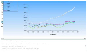
Figure 12: Residual monitor for k and epsilon in ANSYS Fluent. Rising k or ϵ residuals can show unstable turbulence equations.

• Outlet Backflow Problems

Pressure outlets can cause turbulence errors when flow enters the domain from the outlet. This happens in wakes, short domains, and strong recirculation zones. In this case, Fluent uses backflow turbulence values. If these values are not realistic, wrong k and ϵ enter the domain. The error can stay near the outlet or move upstream. A better solution is to move the outlet farther from the main flow region. If this is not possible, set realistic backflow turbulence intensity and length scale.

• Near-Wall Mesh and Wall Treatment

Near a wall, velocity changes rapidly, creating intense shear. If your first cell height is improperly sized, k, ε, and heat transfer predictions will fail.

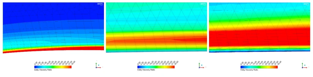
Figure 13: Near-wall mesh and y+ check in ANSYS Fluent. Wall treatment can change k, ϵ, wall shear stress, and heat transfer results.

• Strange k and ϵ Contours

Not all problems create Fluent warnings. Sometimes the solver is stable, but the contours are not physical. A k contour may show high turbulence in a calm zone. An ϵ contour may show sharp peaks in one or two cells. A turbulent viscosity contour may be very high far from the real mixing region.

The location is important. High k in a wake or jet shear layer can be normal. High ϵ near a wall can also be normal. The contour must match the flow physics.

Quick guide for reading k and ϵ contour problems.

Contour Sign	Is It Normal?	What to Check
High k in a wake	Often yes	Check velocity wake and separation
High k only at inlet	Maybe no	Check inlet turbulence intensity
High ϵ near wall	Often yes	Check wall mesh and y+
High ϵ in one cell	Usually no	Check mesh quality
High turbulent viscosity in calm flow	No	Check k, ϵ, and inlet setup
Velocity, k, and ϵ do not match	No	Review setup and boundary conditions

A stable CFD result needs more than low residuals. Check pressure drop, outlet flow rate, force, temperature, and heat flux. If these values still change, the solution is not ready.

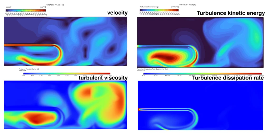
Figure 14: Checking turbulence contours in ANSYS Fluent. Velocity, k, ϵ, and turbulent viscosity should follow the same flow physics.

How to Plot and Read k and ε Contours

Residuals prove numerical stability; contours prove the physics. You must plot Turbulence Kinetic Energy, Turbulence Dissipation Rate, and Turbulent Viscosity.

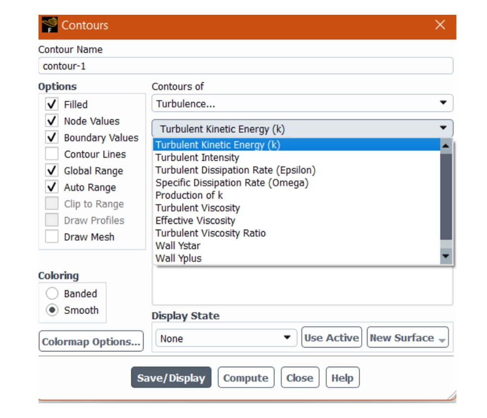
Figure 15: Turbulence variables in ANSYS Fluent post-processing. The user can plot k, ϵ, and turbulent viscosity to check the turbulence field.

High k is common in jet shear layers, wakes behind bodies, recirculation zones, and strong wall shear regions. For example, in a Turbulent Jet in a Cavity CFD Simulation, high k cleanly highlights the mixing boundary between the jet and the ambient fluid.

Figure 16:Turbulent jet in a cavity. The turbulence kinetic energy contour shows strong mixing in the jet shear layer.

Conversely, high ε appears where energy is lost quickly, typically in small cells right against the wall. A sharp ε peak in a single isolated cell away from walls usually indicates a broken mesh element.

When evaluating moving boundaries, such as an Oscillating Cylinders CFD Simulation or a Vortex Induced by Cylinder Vibration, checking these contours at different time steps reveals how the turbulent wake sheds and decays.

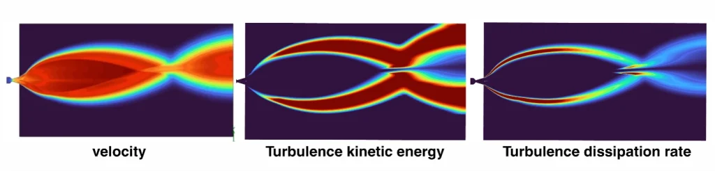
Figure 17: Velocity, k, ϵ, and contours in ANSYS Fluent. These plots should follow the same flow physics.

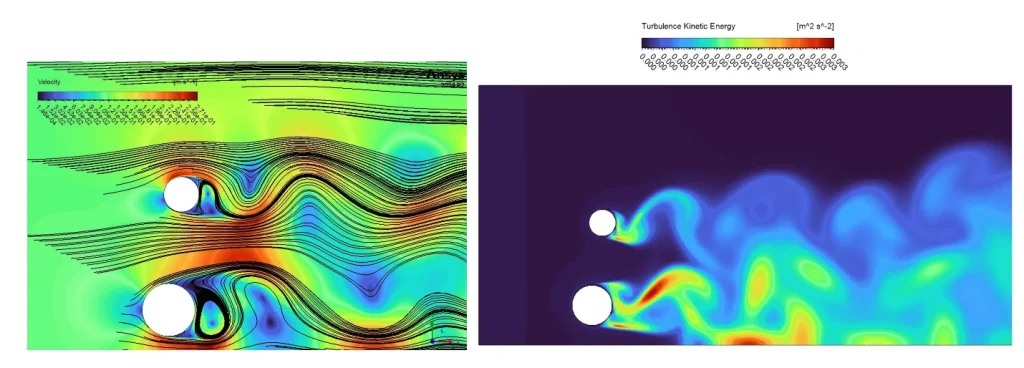
Figure 18: Kinetic energy contour around an oscillating cylinder. The wake changes with body motion and time.

Final Checklist for k and ε Contours

Before accepting your results, verify:

1. Does the high k region align perfectly with the velocity wake or shear layer?
2. Is the turbulent viscosity ratio reasonably low in calm, freestream regions?
3. Are the high ε zones naturally clinging to the walls or high-strain areas?
4. Are the contours smooth, or are there jagged, unphysical spikes?
5. Do the turbulence contours remain stable across multiple iterations?

FAQ About k and ε in ANSYS Fluent

1. What is turbulence kinetic energy in ANSYS Fluent? Turbulent kinetic energy (k) represents the energy of velocity fluctuations. It demonstrates the physical strength of the turbulent motion.

2. What is turbulence dissipation rate? Turbulence dissipation rate (ε) dictates how fast turbulent energy is destroyed by viscosity. It is heavily concentrated near walls and in high-shear zones.

3. Why are k and ε important in the k-epsilon model? The solver uses k and ε to calculate turbulent viscosity (μt). This variable directly governs mixing, pressure drop, and wall shear stress.

4. How should I define k and ε at the inlet? Unless you have precise experimental data, use Intensity and Hydraulic Diameter for internal flows, or Intensity and Length Scale for external free-shear flows.

5. What is a normal turbulence intensity value? Low-turbulence external flows use 1% or lower. General internal flows use 1% to 5%. Fully turbulent pipes use 5% to 10%.

6. Is kinetic energy the same as turbulence kinetic energy? No. Standard kinetic energy relates to the main, averaged flow velocity. Turbulent kinetic energy relates strictly to the chaotic velocity fluctuations. Check the specific variable name in your post-processing tree

7. What should I do if k or ϵ looks wrong? Start with simple checks. Do not change the turbulence model first. Check the inlet turbulence values, hydraulic diameter, mesh quality, outlet backflow, wall treatment, and y+. For wall-related problems, read y+ in CFD and Near-Wall Treatment in ANSYS Fluent Viscous Model.

Figure 19: What Is y+ in CFD? and Near-Wall Treatment in ANSYS Fluent Viscous Model article in CFDLAND

8. What is a normal turbulence intensity value?

There is no single value for all cases. But common engineering values are:

Flow Condition	Typical Turbulence Intensity
Low-turbulence external flow	1% or lower
General internal flow	1% to 5%
Fully turbulent pipe flow	5% to 10%
Strong mixing or disturbed inlet	More than 10%

These values are only starting points. The final choice must match the real flow condition.