
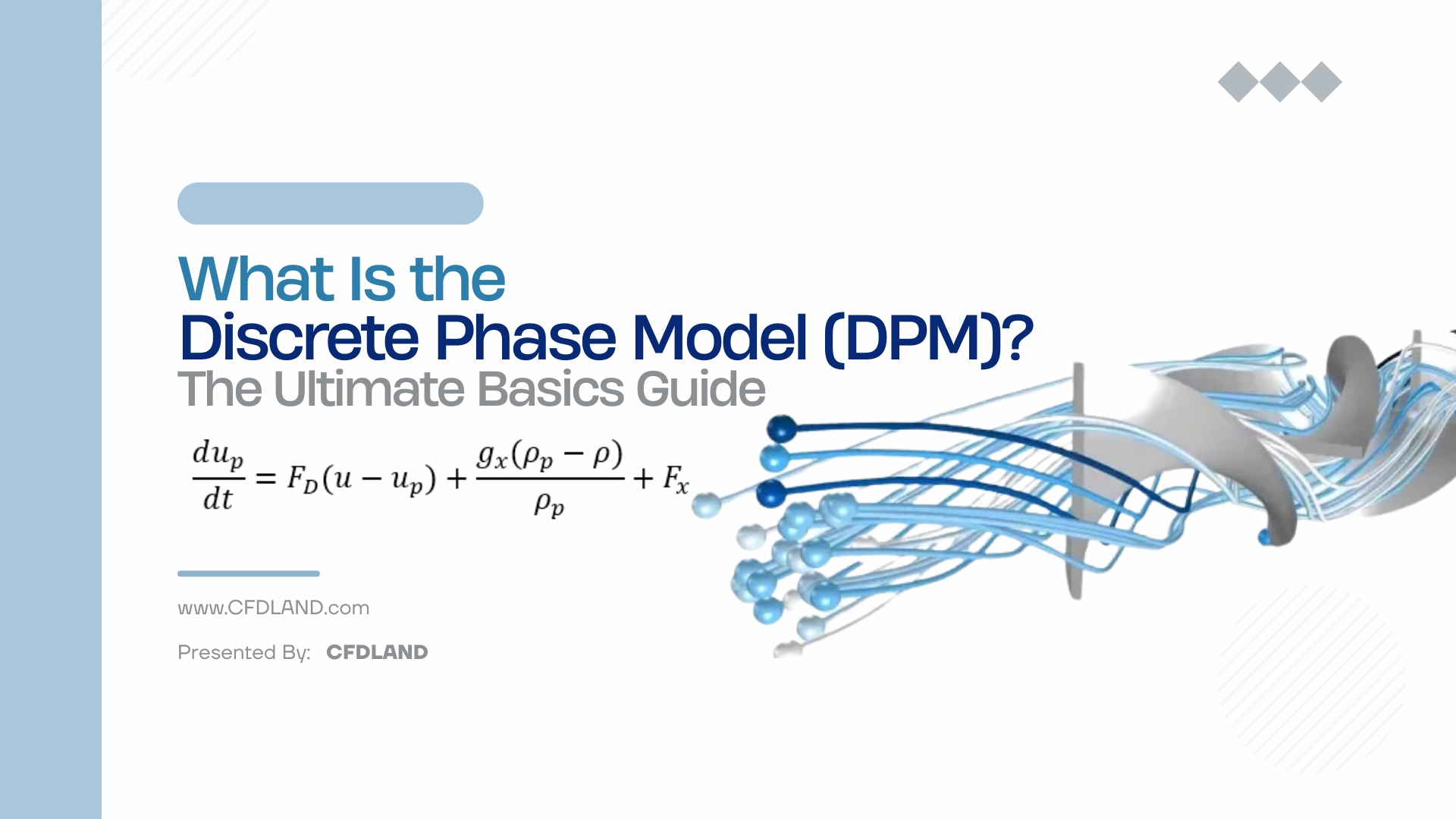
Welcome to the central pillar of our 14–blog path on multiphase DPM simulations. This guide will provide the ultimate technical foundation for particle tracking. However, if you need step-by-step video tutorials to learn in action, please visit our ANSYS Fluent DPM CFD tutorials.
We start by answering a fundamental engineering question: what is Discrete Phase Model? By DPM definition, it is a coupled Eulerian-Lagrangian mathematical approach.
To understand this, we should look at how the software treats the different phases in a system. The software, ANSYS Fluent, divides the problem into 2 separate frameworks:
- First, it solves the continuous phase (such as a flowing liquid or gas) using the standard Eulerian equations on a fixed control volume mesh.
- Second, it handles the dispersed discrete phase (such as solid dust, coal particles, or liquid droplets). Instead of treating this dispersed phase as a continuous cloud, the solver uses Lagrangian particle tracking.
This means Newton’s second law of motion is used to track the physical path of each individual particle as it moves freely through the fluid flow.
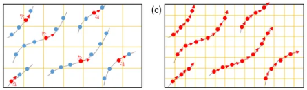
Figure 1: The Discrete Phase Model (DPM) uses a continuous Eulerian field for the fluid flow and Lagrangian tracking for individual particle trajectories.
When to Use the Discrete Phase Model (DPM)
Knowing when to use DPM is essential for an accurate simulation. The most important physical limitation of this discrete phase model in CFD is the volume fraction of the particles.
DPM is specifically designed for highly dilute flows. In our experience, we recommend using this model only when the dispersed phase volume fraction is very low, typically less than 10 to 12% (a volume fraction of 0.1 or less). Because the particles are spread far apart in a dilute flow, the standard mathematical model assumes that particle-particle collisions and interactions are negligible and can be ignored.
This makes the model highly effective for real-world applications such as:
- Liquid droplet evaporation and spray dryers.
- Fuel injection and coal combustion chambers.
- Cyclone separators and particle filtration systems.
- Dust transport and air pollution tracking.
However, DPM is not suitable for dense flows. If your project involves heavy slurry flows, thick sediment transport, or bubbling fluidized beds where the particle volume fraction is very high, the standard model will fail. For those dense conditions, you must switch to Eulerian-Eulerian multiphase models or use advanced dense-phase setups.
DPM vs. Eulerian Multiphase Models
When setting up a multiphase flow simulation, user must choose between different mathematical frameworks. According to academic literature on particle-fluid flows, the 2 most common approaches are the Eulerian-Eulerian method and the Eulerian-Lagrangian method (which is the DPM).
In the Eulerian-Eulerian approach, the software treats both the fluid and the particulate phases as interpenetrating continuous phases. This method is highly effective for dense flows with high volume fractions. However, because it treats the particles as a continuous cloud, it loses the ability to track individual particle details.
When comparing DPM vs Eulerian approaches, the Discrete Phase Model provides a distinct advantage: it tracks individual particles, droplets, or bubbles. This gives user highly detailed data about the trajectory and physical state of each specific particle. The main drawback of DPM is the computational cost. If the physical particle count is extremely high, calculating the path of every single entity requires massive CPU time.
![arrangement of the fluid (blue) and particles (red) in the reservoir. Once with Lagrangian-eulerian and on the right side, a Eulerian-Eulerian approach [Heidler et al.]](https://cfdland.com/wp-content/uploads/2026/07/2.png "image of What Is the Discrete Phase Model (DPM)? The Ultimate Basics Guide")
Figure 2: arrangement of the fluid (blue) and particles (red) in the reservoir. Once with Lagrangian-eulerian and on the right side, a Eulerian-Eulerian approach [Heidler et al.]
Here is a simple summary table comparing the 2 approaches:
| Feature | Discrete Phase Model (DPM) | Eulerian-Eulerian Model |
| Mathematical Framework | Eulerian-Lagrangian | Eulerian-Eulerian |
| Particle Treatment | Individual tracking (discrete) | Interpenetrating continua (cloud) |
| Best Volume Fraction | Dilute flows (< 10 to 12%) | Dense flows (> 12%) |
| Data Detail | High (trajectories) | Low (average phase concentrations) |
| Computational Cost | High (if particle count is large) | Moderate to High (mesh dependent) |
The Core Governing Equation of DPM
To understand how the software tracks these particles, we ought to see the fundamental mathematics. The core governing equation of the discrete phase model in CFD is a simple force-balance equation based on Newton’s second law of motion.
In the Lagrangian reference frame, ANSYS predicts the trajectory of a discrete particle by integrating the forces acting upon it. This equation equates the particle’s inertia with all the physical forces exerted by the continuous fluid stream.
In a standard Cartesian coordinate system, the particle motion equation in the -direction is written as:
\frac{du_p}{dt} = F_D (u - u_p) + \frac{g_x (\rho_p - \rho)}{\rho_p} + F_x
in this equation:
- \frac{du_p}{dt} : This represents the particle acceleration (the inertia).
- F_D(u - u_p) : This represents the drag force per unit particle mass. The variable u is the continuous fluid phase velocity, u_p is the discrete particle velocity, and F_D is the specific drag coefficient.
- \frac{g_x(\rho_p - \rho)}{\rho_p} : This accounts for the gravity and buoyancy forces. Here, rho_p is the exact particle density and rho is the continuous fluid density.
- Fx: This represents any additional physical forces acting on the particle (such as thermophoretic force, virtual mass force, or pressure gradient forces).
For detailed calculations regarding particle velocities and injection flow rates, refer to our Velocity-Flow Rate Relationship Guide.
Key Components of a DPM Setup
For a DPM simulation, we need to configure several specific parameters in the CFD solver. To keep this basic DPM definition clear, we will briefly introduce the 4 main configuration steps.
For clear technical instructions on each step, please follow the links to our blogs:
- Injections: This defines how the particles enter the fluid domain. You can set them to enter as a single particle, a surface release, and many other DPM injection types.
- Particle Types: This setting defines the physical state and behavior of your discrete phase. Common selections include Inert solid particles, evaporating Droplets, or Combusting particles. So you should know all particle types given by software.
- Boundary Conditions: This determines how particles react mathematically when they impact the physical walls of your geometry. The standard reactions are Reflect, Trap, and Escape. There are also more complicated DPM boundary conditions for special applications.
- Physical Sub-Models: This tab allows you to activate additional physical forces and phenomena acting on the particles, such as thermophoretic forces or boiling.
Conclusion & Next Steps
This is the first step to simulate complex multiphase systems. By understanding what is Discrete Phase Model and how Lagrangian particle tracking operates, you now have the academic foundation needed to build accurate and reliable computational models.
If you are ready to apply these concepts to industrial problems, or if you require professional engineering consulting for your specific system, we are here to help. Please visit our DPM CFD Simulation Category mentioned in the introduction to explore our capabilities, or head directly to our Project Ordering page to submit your geometry and requirements for a verified simulation model.