Optimization Algorithms in ANSYS: From NLPQL to MOGA

If you read our first article, The Complete Guide to Optimization in ANSYS, you know the basic concepts of structural and fluid optimization. In our second article, Design of Experiment (DOE) & Response Surface Methodology (RSM) in ANSYS, we explained how to build a mathematical model of your system. Now, we must use an algorithm to search that model and find the optimum point.

This final step uses ANSYS optimization algorithms. These mathematical engines process the inputs and outputs to achieve your specific design goals. Because there are many different mathematical approaches, selecting the correct algorithm is essential for success. Some algorithms are built for speed, while others are designed to handle highly complex, noisy data. In this blog, we will explain how these algorithms work and when to use them. For practical simulation examples, you can explore our library of ANSYS Optimization Tutorials.

Figure 1: The standard flowchart for a single objective optimization problem involves exploring the design space before applying a mathematical optimization algorithm.

The Optimization Setup

Before any optimization algorithm can find the best design, you must define the mathematical rules of your problem. In ANSYS, this setup acts as the foundation for the solver. If the setup is wrong, the algorithm will not find a useful result. To create a proper framework, you must define 3 main components: variables, objectives, and constraints.

• Defining Design Variables: Design variables are the input parameters that the algorithm is allowed to change. You must set a specific range for each variable by defining a lower bound and an upper bound. Variables can be continuous, meaning they can take any decimal value between the bounds. They can also be discrete, meaning they can only take specific predefined values.
• Defining Objective Functions: The objective function is the ultimate goal of your study. You must tell the algorithm what you want to achieve with your output parameters. You can set the solver to minimize or maximize a specific value. For example, a common engineering goal is to minimize the mass of a structure or maximize the fluid velocity in a pipe. You can also target a specific value.
• Defining Constraints: Constraints are the strict rules of the system. While the algorithm tries to achieve the objective, it must not violate the constraints. For example, you want to minimize the mass, but the maximum stress must stay below the yield limit of the material. In ANSYS, you define these rules using inequality constraints, such as ensuring a value is less than or greater than a specific limit.

Figure 2: The optimization setup requires clear objective functions and strict inequality constraints to guide the algorithm.

Once these 3 components are defined, the design space is ready. The algorithm will now use this map to evaluate different designs and find the optimum point.

Direct vs. Response Surface Optimization

When you run an optimization algorithm in ANSYS, you must make a major decision about how the solver evaluates the designs. You must choose between Direct vs Response Surface Optimization.

On one side, In direct optimization, the optimization algorithm connects directly to the high-fidelity simulation. The optimizer requests a new design point, the real simulation runs, and the result is sent back to the optimizer.

• Advantages: This method is highly accurate because it always uses the physics of the real simulation. It does not introduce any approximation errors.
• Disadvantages: It requires a very high computational cost. If your CFD or FEA simulation takes 4 hours to run, testing 100 design points is often impossible. Direct methods can also fail easily if the simulation has small numerical noise.

On the flip side, in response surface optimization, the software replaces the slow simulation with a fast mathematical approximation model. First, the software tests a small set of sample points. Then, it builds a smooth mathematical surface. The optimizer searches on this artificial surface instead of running the real simulation.

• Advantages: Because the mathematical surface is a simple equation, evaluating thousands of designs takes only a few seconds. The smooth surface also filters out numerical noise automatically.
• Disadvantages: It is only an approximation. If the mathematical model has errors or poor training data, the optimizer might predict a false optimum or miss the true best design entirely.

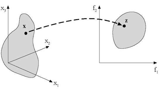
Figure 3: The choice between direct and response surface optimization determines how the software maps the design space into the objective space.

Single-Objective: Gradient-Based Methods

Gradient based optimization methods are algorithms used for single objective optimization. They calculate the local slope, or gradient, of the objective function to find the lowest or highest point. You can imagine this as walking down a mountain by always taking the steepest path down. In ANSYS, two of the most important gradient-based methods are NLPQL and MISQP.

NLPQL

NLPQL stands for Non-Linear Programming by Quadratic Lagrangian. It is a highly efficient algorithm for smooth problems. If your objective function is smooth and you only have continuous variables, NLPQL will find the optimal design very quickly. However, NLPQL has strict limitations. It cannot solve problems with discrete variables. Also, if your solver produces noisy data with small artificial bumps, the algorithm might get stuck in a false local minimum.

Figure 4: Gradient-based methods like NLPQL use the local slope of the function to quickly calculate the next step toward the optimum design. [Kelley, C. T. 1999. Iterative Methods for Optimization. Philadelphia: Siam, Society for Industrial; Applied Mathematics]

MISQP

MISQP stands for Mixed-Integer Sequential Quadratic Programming. It is an advanced version of the standard NLPQL method. The main advantage of MISQP is its ability to handle mixed problems. This means it can optimize a system that has both continuous variables and discrete variables (such as manufacturable material thicknesses like 5 or 6). While MISQP is very powerful, it still relies on local gradients. Therefore, it requires a very good starting point to find the true global optimum.

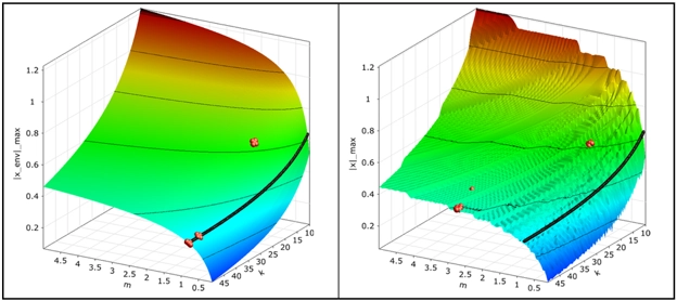
Figure 5: NLPQL converges perfectly on smooth functions but can fail or get stuck if the objective function contains numerical noise.

Single-Objective: Pattern Search Methods

Pattern search methods do not use mathematical gradients to find the best design. Instead, they use a geometric pattern of points to explore the space. Because they do not calculate local slopes, they work very well when your objective function is noisy or discontinuous.

Downhill Simplex

The Downhill Simplex method is a direct search algorithm. It uses a simple geometric shape called a simplex. In a 2-dimensional problem, this shape is a triangle. The algorithm evaluates the corners of the shape. It finds the worst point and replaces it with a better one. It does this by reflecting, expanding, or shrinking the shape. It is a very stable method, but ANSYS recommends it only for problems with up to 5 input variables.

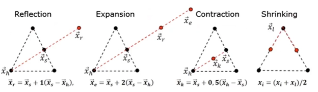
Figure 6: The Downhill simplex method moves toward the optimum design by reflecting or shrinking its geometric shape away from the worst points.

IRECT and Pattern Search

The DIRECT method stands for DIviding RECTangles. It searches the design space by dividing it into smaller and smaller boxes. It evaluates the center of each box to find the minimum value. This method is excellent because it balances local search and global search at the same time. Other similar methods include the Hooke-Jeeves pattern search, which tests points by taking small steps in each direction.

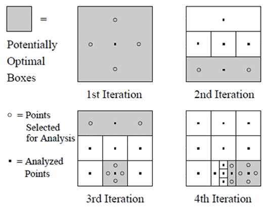
Figure 7: The DIRECT algorithm divides the design space into smaller rectangles to mathematically balance global exploration and local search.

Single-Objective: Response-Surface-Based

Response surface-based methods use a mathematical approximation instead of the real solver. To make this process accurate, ANSYS uses adaptive algorithms. These methods automatically improve the mathematical surface during the optimization to ensure the final result is correct.

ARSM

The ARSM (Adaptive Response Surface Method) builds a local polynomial model. It finds the optimum on this small surface. Then, it creates a new, smaller design space around that point. It repeats this process until the box shrinks to the final answer. Because it uses many points to build the local surface, it is very stable against solver noise.

ASO

The ASO (Adaptive Single-Objective) method is a highly advanced tool in ANSYS. It uses a Kriging response surface and the MISQP algorithm. First, it searches the surface to find a candidate point. Then, it uses a built-in error predictor to check if the point is reliable. If the predicted error is too high, it runs a real simulation to improve the Kriging surface. If the error is low, it accepts the design. This method is incredibly fast and smart.

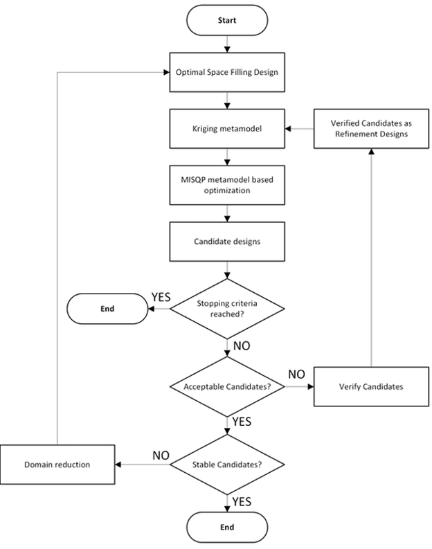
Figure 8: The Adaptive Single-Objective (ASO) workflow continuously checks its own accuracy and updates the Kriging surface only when necessary.

EGO and Bayesian Optimization

EGO (Efficient Global Optimization) uses Bayesian logic. It does not just look for the lowest predicted value. Instead, it calculates the Expected Improvement. This means it looks at both the predicted best value and the mathematical uncertainty of the model. It automatically decides whether to explore a new unknown area or to exploit a known good area.

Figure 9: Bayesian optimization uses the model’s uncertainty to find the areas that offer the highest expected improvement for the objective function. [Bayesian Optimization for Accelerating Hyper-Parameter Tuning]

Single-Objective: Nature-Inspired Methods

Nature inspired optimization methods copy natural processes like biological evolution or swarm intelligence. They do not use mathematical gradients. Instead, they use a large group of artificial individuals to search the design space.

The algorithm starts with a random population. It tests each individual and assigns a fitness score. A better score corresponds to a smaller objective value. The software keeps the best designs and creates a new generation. This cycle repeats until the solver reaches the maximum number of iterations. These methods are excellent for highly complex problems, discrete variables, and noisy data where gradient methods fail.

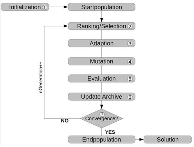
Figure 10: Nature inspired algorithms evaluate the fitness of a population and use selection methods to create better generations over time.

Evolutionary Algorithms (EA)

Evolutionary Algorithms (EA) are search methods that imitate natural biological evolution. They use parent selection, crossover, and mutation to create new offspring designs. ANSYS provides several variations of these algorithms. The Darwin algorithm is a genetic search tool that easily handles discrete variables and penalizes constraint violations. Another advanced version is the Covariance Matrix Adaptation (CMA). It is an evolution strategy designed for continuous problems. The CMA algorithm learns the sampling distribution automatically without requiring derivative data. It is recommended for problems with up to 20 variables.

Particle Swarm Optimization (PSO)

This imitates the social behavior of a bird flock or fish school. Every individual particle remembers its personal best position. It also knows the global best position found by the entire swarm. The movement of each particle depends on 3 main parameters. The inertia weight controls the previous speed. The personal acceleration coefficient pulls the particle toward its own best memory. The global acceleration coefficient pulls the particle toward the swarm’s best location. This method is highly accurate for continuous variables but can be slower than evolutionary methods if you have many constraints.

Stochastic Design Improvement (SDI)

It is a local optimization procedure. It randomly generates a sampling scheme around the best design of the previous iteration. It does not require extensive knowledge about the design space. Because it relies on a pure random approach, it is highly useful if your simulation has a large number of failed designs.

Adaptive Simulated Annealing (ASA)

It copies the metallurgical cooling process. The search starts with a high temperature parameter. At this stage, the solver accepts worse designs with a high probability. This allows the solver to escape false local minima. As the optimization progresses, the temperature slowly drops. The search area becomes smaller, and the solver focuses on finding the global minimum.

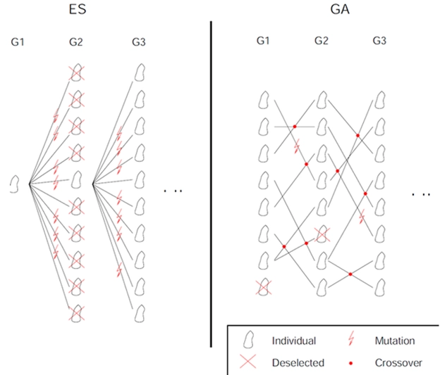
Figure 11: Evolutionary Algorithms apply mathematical crossover and mutation to create offspring from the best parent designs.

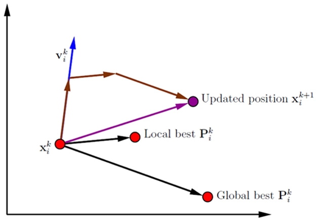
Figure 12: The Particle Swarm Optimization algorithm moves candidate designs by balancing their personal best experience with the swarm’s global best discovery.

The Pareto Concept

In optimization problems, we often have different goals at the same time. Sometimes, improving one goal makes another goal worse. This is a conflicting objective. For example, if you want to minimize the mass of a car part, you might accidentally increase the stress on that part. You cannot have perfect results for both.

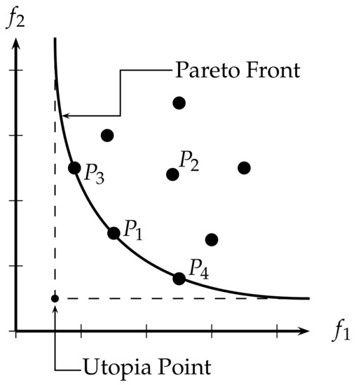
Figure 13: the Pareto front shows the set of best compromise designs where no single objective can be improved without hurting another.

The Pareto Concept helps us solve this problem. People often call it the 80/20 rule. It states that roughly 80 percent of the consequences come from 20 percent of the causes. In the context of efficiency, this rule helps you find the most important inputs. By finding the vital few parameters, you can focus your time and money on the changes that give the biggest impact.

In ANSYS, this concept is the mathematical foundation of multi objective optimization. The software looks for special designs called Pareto optimal solutions. A design is Pareto optimal if you cannot improve one objective without making another objective worse. It is the absolute best compromise between your conflicting rules.

When the algorithm finishes searching the objective space, it plots all of these optimal candidate points on a graph. The points connect to form a boundary curve. This curve is called the Pareto front. Instead of giving you just 1 perfect answer, the software gives you a family of best answers on this front. We must look at the Pareto front and select the final design that best fits the project needs.

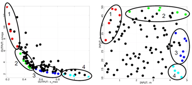
Figure 14: Engineers analyze the Pareto front to understand conflicting objectives and select the final optimal design for their project.

Multi-Objective: Classic Methods

Classic multi-objective methods do not search the entire Pareto frontier directly. Instead, they use mathematical tricks to convert the multi-objective problem into a simple single-objective problem. ANSYS provides 2 classic methods for this task.

Weighted Sum

The Weighted Sum method is the most common approach. It combines all your different objectives into 1 single function. It does this by multiplying each objective by a specific weight factor. For example, you can give a 70 percent weight to the mass and a 30 percent weight to the stress. This method is very simple and easy to use. However, it has limitations. If your objective space has a non-convex shape, this method cannot find certain optimal solutions. Also, mixing different types of goals, like minimizing and maximizing at the same time, requires extra mathematical conversions.

ε-Constraint

This method uses a different approach. It keeps only 1 main objective and changes all the other objectives into strict constraints. For example, it will minimize the mass, but it will force the stress to stay strictly below a specific ε limit value. This method works well for both convex and non-convex problems. However, the engineer must choose the ε limit values very carefully to find a valid solution.

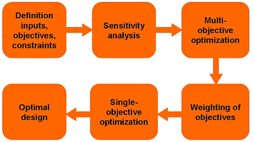
Figure 15: Classic methods often require engineers to use sensitivity analysis to identify conflicting objectives before applying weights or constraints.

Multi-Objective: Key Algorithms

To find the best designs on the Pareto front, ANSYS uses advanced genetic algorithms. These methods search the objective space and keep the best designs over many generations. The 2 most important tools for this task are NSGA-II and MOGA.

NSGA-II

NSGA-II stands for Non-dominated Sorting Genetic Algorithm II. It is designed to find a diverse set of answers on the Pareto front. First, it uses a fast mathematical sorting method to rank all designs. Next, it uses elitism. Elitism means the algorithm copies the absolute best designs from the old generation directly into the new generation so they are never lost. Finally, to keep the answers diverse, it uses a crowding distance operator. This operator forces the algorithm to spread the designs out, preventing it from putting all the answers in 1 small spot.

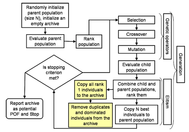
Figure 16: The NSGA-II method uses elitism to ensure the best non-dominated solutions are never lost during the search.

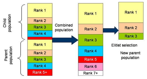
Figure 17: Elitism in NSGA-II

MOGA

MOGA stands for Multi-Objective Genetic Algorithm. It is a faster, upgraded hybrid version of NSGA-II. It uses controlled elitism to manage the designs. MOGA is unique because it does not use mathematical penalty functions if a design violates a constraint. Instead, it uses the same dominance rule for constraints and objectives. This forces the solver to always rank feasible designs higher than infeasible ones. The algorithm also saves the first optimal designs in a separate archive to protect the early patterns of the Pareto front.

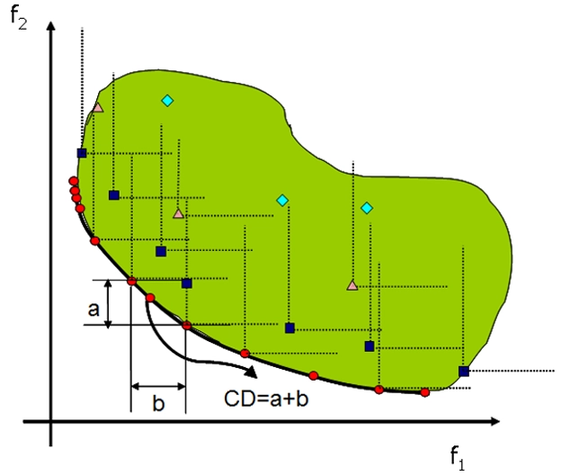
Figure 18: Both NSGA-II and MOGA use crowding distance calculations to maintain a diverse spread of designs across the Pareto front.

Reading Results

After the optimization finishes, you must analyze the visual data. ANSYS DesignXplorer provides several specific charts and tables for post-processing. You must read these visual tools carefully to select your final optimal design.

Candidate Points Table

The software does not give just 1 answer. It provides a table of the best candidate points. This visual table lists the values for all inputs and outputs. It compares the mathematical approximated values (often in blue text) with the real verified values (in black text). The table uses a visual rating system. It gives up to 3 gold stars to show how well a candidate meets your design goals.

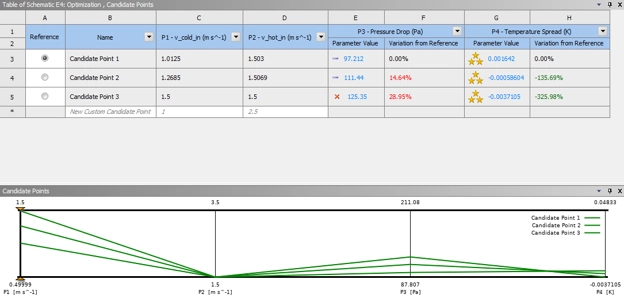
Figure 19: The candidate points table uses visual star ratings to help engineers easily identify the best designs.

Tradeoff Chart

The tradeoff chart is a visual map of the objective space. It plots the candidate points on a graph to form a boundary curve. This curve is the Pareto front. You can view this chart in 2D or 3D. This visual data helps you easily see how reducing the a variable will directly change the other variables.

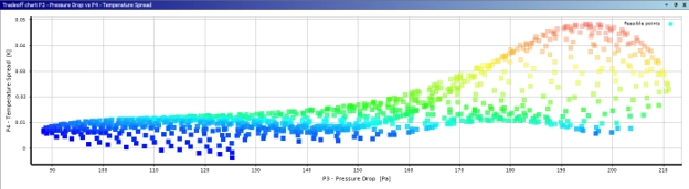
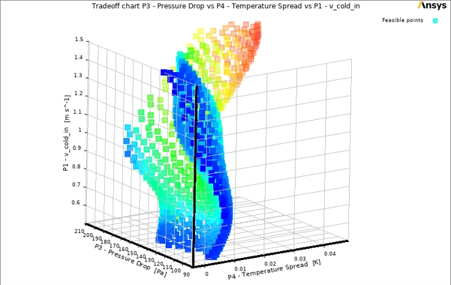
Figure 20: The tradeoff chart visually maps the objective space in 3D to display the exact Pareto front curve.

Sensitivities Chart

This visual chart shows which input parameters drive your outputs. It presents the data as a bar chart or a pie chart. A positive bar means increasing the input increases the output. A negative bar means increasing the input decreases the output. This visual helps you identify and ignore unimportant parameters.

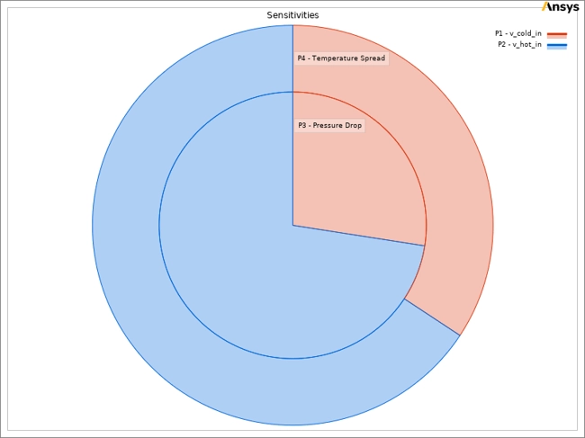
Figure 21: In this example, it`s the velocity of hot inlet that derives the performance

Parameters Parallel Chart

This chart displays parallel vertical axes for all parameters. Every single design point is a colored line that crosses these vertical lines. The top and bottom of each axis show the maximum and minimum values. It provides a complete visual flow of data from inputs to outputs.

Conclusion

In this final part of our 3-blog series, we explored the most advanced mathematical tools in ANSYS. We started with single objective methods like pattern search and response surface algorithms. Then, we explained the Pareto concept for handling conflicting goals. Finally, we looked at multi objective methods such as MOGA and NSGA-II. These powerful algorithms evaluate the objective space and help you find the absolute best candidate points for your engineering projects.

Note: This blog is written mainly based on official ANSYS documents, and the images are taken mainly from it. We tried to simplify the text and extract the essential things to help you easily understand the physics and mathematics behind the software.