
Simulating particulate flows requires a deep understanding of how solid materials behave inside a continuous fluid. Depending on the concentration of the solids, particles will either fly freely without touching, or they will constantly crash and rub against each other in dense zones.
ANSYS Fluent provides several distinct mathematical approaches to accurately capture these complex physics. Your choice strictly depends on how heavily the particles interact and whether you need to track individual discrete particles or treat the entire solid mass as a continuous fluid.
Choosing the incorrect multiphase model will completely ruin your simulation, either by ignoring critical particle collisions or by requiring computationally impossible solving times.
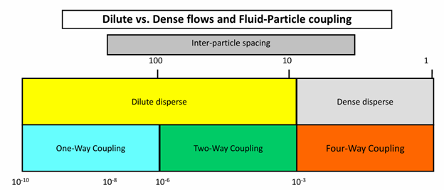
Figure 1: Selecting the correct multiphase approach strictly depends on the solid concentration and the mathematical nature of the particle-particle interactions.
Some models use a strict Eulerian-Eulerian approach, where the fluid and the solids are treated as interpenetrating fluids. Other advanced models use an Eulerian-Lagrangian approach, where the fluid is a standard flow field, but the solids are tracked as millions of individual moving points. If you want to master these setups practically, we highly recommend exploring our comprehensive Multiphase CFD Simulation Tutorials.
Based directly on the ANSYS multiphase guidelines, here is a highly detailed comparison table of all available particulate modeling approaches to help you make the absolute best choice:
| Model | Numerical Approach | Particle-Fluid Interaction | Particle-Particle Interaction |
| Discrete Phase Model (DPM) | Fluid: Eulerian Particles: Lagrangian |
Empirical models for sub-grid particles | Completely neglected. |
| DDPM-KTGF | Fluid: Eulerian Particles: Lagrangian |
Empirical models for sub-grid particles | Approximate interactions determined by granular models. |
| DDPM-DEM | Fluid: Eulerian Particles: Lagrangian |
Empirical models for sub-grid particles | Accurate, explicit determination of physical collisions. |
| Macroscopic Particle Model | Fluid: Eulerian Particles: Lagrangian |
Interactions determined as part of solution (particles span many cells). | Accurate, explicit determination of physical collisions. |
| Euler Granular Model | Fluid: Eulerian Particles: Eulerian |
Empirical models for sub-grid particles | Modeled entirely by fluid properties like granular pressure and viscosity. |
Dense Discrete Phase Model (DDPM)
The standard Discrete Phase Model (DPM) is an incredibly popular tool for simulating particles, but it has a massive mathematical limitation. It strictly assumes the flow is dilute, meaning the particles will never crash into each other and they do not take up any physical space in the fluid. If your solid concentration increases, standard DPM will produce completely invalid and unphysical results.
To solve this severe limitation, ANSYS Fluent provides the Dense Discrete Phase Model (DDPM). This advanced framework solves the continuous fluid on a standard Eulerian mesh while strictly tracking the solid phase as discrete points in a Lagrangian frame.
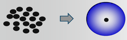
The true power of the Dense Discrete Phase Model in ANSYS Fluent is that it explicitly calculates the physical volume fraction of the particles, allowing you to accurately simulate highly concentrated, heavy particulate flows.
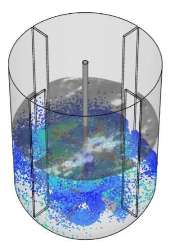
Figure 2: The Dense Discrete Phase Model (DDPM) extends traditional Lagrangian tracking by accounting for the physical space particles occupy, making it perfect for highly concentrated flows.
Because DDPM recognizes how much physical space the particles occupy, it mathematically forces the fluid to accelerate as it squeezes through the tight gaps between the solids. It also strictly accounts for the mass, momentum, and energy exchange between the fluid and the particles. Furthermore, because it uses Lagrangian tracking, DDPM can effortlessly handle a very wide Particle Size Distribution (PSD) without requiring you to create dozens of different fluid phases.
This multiphase capability makes DDPM the ultimate choice for heavy industrial applications. For example, in our Industrial Cyclone Preheater CFD Simulation Using DDPM in Fluent, we utilize this exact model to capture the complex turbulent swirling gas-particle flow. Similarly, DDPM is not limited only to gas-solid flows; it is exceptionally powerful for liquid-solid systems as well. We successfully apply this in our Particle Mixing CFD: A DDPM Fluent Tutorial for Mixer Tank Simulation. In this complex three-phase project, DDPM perfectly captures the highly concentrated slurry formation at the bottom of the tank and predicts the severe velocity gradients created by the impeller.

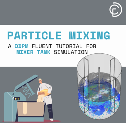
Figure 3: Two famous examples of DDPM in CFDLAND projects
DDPM Solution Procedure
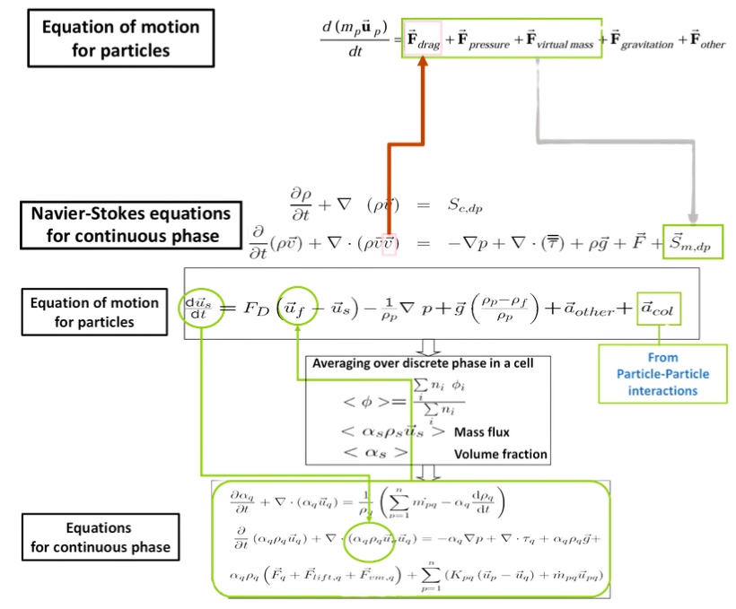
To accurately simulate these dense flows, ANSYS Fluent uses a very specific two-step mathematical procedure. First, the solver calculates the standard Navier-Stokes equations for the continuous fluid phase. This firmly establishes the overall velocity and pressure field of the carrier gas or liquid moving through the geometry.
Next, the solver switches its focus to the discrete solid particles. It calculates the explicit equation of motion for each individual flying particle. The software adds up all the aerodynamic drag, gravity forces, and pressure gradients to determine exactly where each particle will travel next.
The real magic of DDPM happens during the cell averaging step, where the software calculates the exact mass flux and volume fraction of the particles inside every single fluid cell.
Instead of simply ignoring the volume of the particles, the solver maps the discrete particle data directly back onto the continuous Eulerian fluid grid. This continuous back-and-forth mapping ensures the heavy particles actively push back against the fluid flow, creating a highly stable and physically accurate two-way coupling effect.
DDPM-KTGF Approach
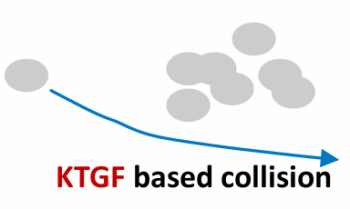
In many industrial simulations, calculating every single physical crash between millions of particles takes too much time and computer power. When your flow is dilute to moderately dense, you can use a much faster mathematical method called the DDPM-KTGF approach.
KTGF stands for the Kinetic Theory of Granular Flow. Instead of explicitly tracking exactly how two individual particles bounce off each other, this model uses approximate mathematical equations. It treats the random, chaotic movement of the solid particles similar to how gas molecules move and collide.
To mathematically predict these collisions, the KTGF model calculates a “Granular Temperature,” which represents the kinetic energy of the bouncing particles using either a simple algebraic formula or particle statistics.
Because the model uses these mathematical approximations to define the solid stress tensor, DDPM-KTGF solves significantly faster than other dense flow models. It allows you to predict particle interaction effects accurately without requiring the massive computational cost of explicit tracking. Furthermore, this approach remains fully compatible with advanced Fluent features like species transport and char combustion frameworks.
Discrete Element Method (DEM)
While the KTGF approach approximates collisions to save time, some complex engineering problems demand absolute physical accuracy. When you need to know exactly how every single particle crashes, rolls, and slides against others, you must use the Discrete Element Method (DEM).
To simulate these highly physical impacts, ANSYS Fluent utilizes the Soft-Sphere Approach. In this mathematical model, particles are not treated as perfectly indestructible rigid points. Instead, when two discrete particles crash into each other, the software allows their geometric boundaries to slightly overlap.
In the Discrete Element Method, this calculated physical overlap acts as a direct mathematical measurement of the particle deformation during a crash. To accurately calculate exactly how the particles bounce off each other, the DEM solver uses three specific contact force laws:
| Force Law | Physical Meaning | Simulation Function |
| Spring Force | Linear Repulsive Force | Pushes the crashing particles away from each other based on a defined Spring Constant. |
| Dashpot Force | Linear Dissipative Force | Absorbs the impact energy based on the Coefficient of Restitution, preventing particles from bouncing forever. |
| Friction Force | Coulomb Friction Law | Calculates the tangential sliding and rubbing resistance based on the surface friction coefficient. |
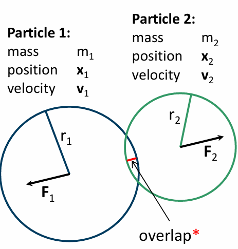
Figure 4: The Discrete Element Method (DEM) calculates explicit collisions by measuring the microscopic overlap between colliding particles to determine the exact spring and dashpot forces.
Based on this overlap, the software calculates massive explicit N-body interactions. To see how these complex collision physics are perfectly set up and solved in industrial software, we highly recommend reviewing our extensive library of DEM CFD simulation tutorials.
DDPM-DEM Approach
The true ultimate capability of ANSYS Fluent multiphase modeling is combining the fluid solving power of DDPM with the extreme collision accuracy of DEM. This is formally known as the DDPM-DEM Approach. By coupling these two mathematical frameworks, the continuous fluid pushes the particles through standard aerodynamic drag, while the Discrete Element Method explicitly calculates every resulting dense physical collision. This combined approach is completely compatible with complex thermal physics, such as char combustion, species transport, and severe heat transfer.
The DDPM-DEM approach provides the absolute highest level of physical accuracy for dense particulate flows, though it requires significantly more computational time to explicitly solve millions of crashes.
Because of its unparalleled accuracy, engineers heavily rely on this coupled model for complex thermodynamic processes where particle rubbing and mixing directly affect thermal efficiency. A perfect demonstration of this is our Drying Grains CFD Simulation: A DDPM-DEM Coupling Tutorial in ANSYS Fluent. In this advanced multiphase project, the explicit DEM collisions perfectly calculate the dense packing of the grains, while the DDPM fluid handles the complex thermal drying gas flowing between the tight gaps.
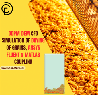
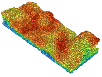
Figure 5: Coupling DDPM with DEM allows engineers to accurately simulate extreme physical scenarios, such as the thermal drying of densely packed grain particles.
Parcels Concept in DEM
In real-world industrial applications, a reactor might contain billions of individual tiny particles! Trying to track the explicit position and collision of every single one of those particles would crash even the strongest supercomputers. To solve this major hardware limitation, ANSYS Fluent uses the Parcels Concept.
Instead of tracking every single grain of sand, the software groups several particles with the exact same properties together into one single “parcel.” The solver then only tracks this one representative super-particle as it flies through the domain. The most critical rule of the parcel concept in DEM is that the mathematical mass used during a collision is the mass of the entire parcel, not just a single particle.
The software calculates the physical radius of the parcel directly from this combined mass and the base particle density. This clever mathematical trick ensures that when these parcels crash and stack up at the bottom of a tank, they still produce the absolutely correct physical volume fraction for sphere packing.
DDPM-KTGF Setup in Fluent
Setting up the DDPM-KTGF approach in ANSYS Fluent requires a very strict sequence of settings to ensure the continuous fluid and the discrete solid phases couple correctly. You must carefully configure the physics in both the general multiphase models window and the specific discrete phase injection menus.
Because the Kinetic Theory of Granular Flow (KTGF) mathematically approximates collisions to save computing time, you only need to define a single discrete phase, even if you are simulating a very wide Particle Size Distribution (PSD). The most critical rule when setting up your multiphase simulation is that you must choose either the KTGF mathematical approximation or explicit DEM physical collisions; ANSYS Fluent will absolutely not allow you to use both simultaneously!
To perfectly configure this specific granular model, engineers must strictly follow a simple three-step procedure inside the software interface:
| Configuration Step | Action Required in ANSYS Fluent | Engineering Purpose |
| Step 1: Enable DDPM | Activate the DDPM model, select the correct fluid-particle drag force, and choose “KTGF” under the Particle-Particle Interaction option. | This tells the solver to track discrete particles but mathematically account for their dense volume fraction. |
| Step 2: Enable Granular Model | Open the Secondary Phase panel and check the “Granular” option. | This actively turns on the Kinetic Theory equations, allowing the solver to calculate granular temperature and solid stresses. |
| Step 3: Define Injections | Create a DPM injection, input the mass flow rate, and strictly assign your created granular phase to this injection. | This physically introduces the discrete parcels into the computational domain linked to the KTGF physics. |
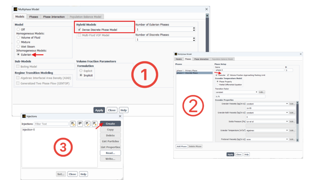
Figure 6: Setting up the DDPM-KTGF model requires activating the granular phase options and strictly assigning them to your discrete particle injections.
DDPM-DEM Setup in Fluent
If your project requires explicit collision tracking, you must set up the DDPM-DEM approach instead. This workflow is slightly different and requires establishing strict mathematical rules for how different materials crash into each other. Just like before, the first step is to enable the DDPM model in the Eulerian multiphase panel. However, for the second step, you completely ignore the granular secondary phase settings. Instead, you directly enable the “DEM” option inside the main Discrete Phase Model (DPM) panel.
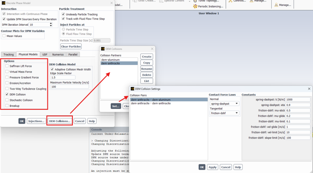
Figure 7: Setting up DDPM-DEM requires defining explicit Collision Partners and assigning precise spring and friction properties for every material pair.
The third step is creating your particle injection. When DEM is active, Fluent will automatically ask you to assign a “Collision Partner” to your injection. A collision partner is essentially a mechanical profile that tells the software exactly how this specific group of particles will behave during a physical impact.
The most critical step in DEM setup is defining the collision properties between pairs of collision partners to calculate exact physical bouncing and sliding.
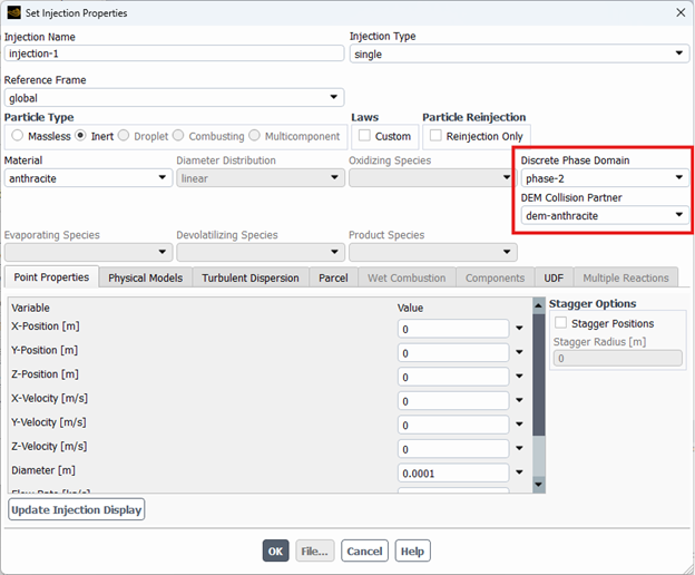
Figure 8: Collision partner suggestion in Injection panel
To help you perfectly configure these complex mechanical interactions, here is a quick-guide table of the required DEM collision property models:
| Collision Property | Mathematical Function | Setup Strategy in Fluent |
| Spring Constant (K) | Determines particle rigidity. | Start with lower values (e.g., 100-1000 N/m) for softer parcels to maintain stable computation. |
| Coefficient of Restitution | Controls energy loss during a crash. | Set between 0 (perfectly sticky) and 1 (perfectly elastic bounce) based on your material. |
| Friction Coefficient | Determines surface sliding resistance. | Defines how easily particles roll over each other; essential for simulating realistic material packing. |
| Collision Pairs | Defines interactions between different materials. | You must explicitly define how “Partner A” collides with “Partner A”, and how “Partner A” collides with “Partner B”. |
DEM Collision Mesh
When calculating explicit DEM collisions, mathematically checking every single particle against every other particle in the domain requires an impossible amount of computing power. To completely solve this bottleneck, ANSYS Fluent automatically generates a hidden framework called the Cartesian Collision Mesh.
Instead of scanning the entire geometry, the software intelligently bins every moving parcel into a localized grid. The solver then evaluates physical crashes exclusively for particles located inside the exact same bin or immediately touching neighboring bins. Fluent automatically adapts the width of this collision mesh based on your largest defined parcel diameter multiplied by an edge scale factor. To ensure this collision tracking works flawlessly, you must configure very specific mathematical parameters inside the Discrete Phase Model (DPM) panel.
The absolute most critical rule for DEM is that your Particle Time Step must be set strictly smaller than the mechanical Collision Time Scale (), otherwise colliding particles will simply pass through each other.

Figure 9: DEM important collision parameters in Discrete Phase Model (DPM) panel.
Because explicitly resolving a micro-second particle crash requires an incredibly tiny time step, engineers use clever mathematical tricks to safely speed up the simulation. Instead of using perfectly rigid steel or glass properties, you can define mathematically softer parcels by lowering the Spring Constant (K) to around 100 – 1000 N/m. Softer parcels absorb impacts smoothly, which allows you to safely increase your particle time step without crashing the solver! Furthermore, your mathematical parcel size must always remain physically smaller than the Eulerian fluid cell it occupies. If multiple large parcels squeeze into a single tiny cell, the local fluid volume fraction artificially drops to zero, causing immediate divergence.
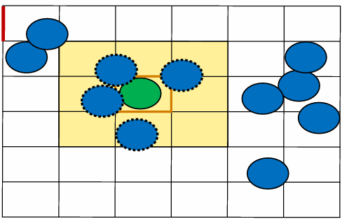
Figure 10: ANSYS Fluent automatically generates a Cartesian Collision Mesh to isolate particle calculations, preventing the solver from wasting time checking distant particles.
To give you a perfect step-by-step setup strategy, here is exactly where to find and set these essential parameters in ANSYS Fluent:
| Parameter & Location in Fluent | Physical Function | Recommended Best Practice Value |
| Node-Based Averaging (DPM Panel > Numerics Tab) | Prevents the fluid volume fraction from hitting zero when dense parcels pack tightly into a single mesh cell. | Always Enable. This smoothly distributes the parcel volume across the neighboring mesh nodes to guarantee solver stability. |
| Particle Time Step (DPM Panel > Tracking Tab) | Determines how often the solver calculates the physical position and overlap of the moving discrete particles. | Specify multiple particle time steps per fluid time step. It must remain smaller than the collision time scale. |
| Max Particle Velocity (DPM Panel > Numerics Tab) | Limits extreme unnatural bouncing if a high-speed collision occurs in the Cartesian mesh. | Enable and set a physically plausible maximum speed. Note: This requires activating the Implicit Tracking Scheme! |
| Spring Constant (K) (DEM Collision Partner Window) | Defines the rigidity of the particles during the explicit soft-sphere overlap calculation. | Start with K = 100 to 1000 N/m. Using softer values prevents mathematical explosion and drastically speeds up calculation time. |
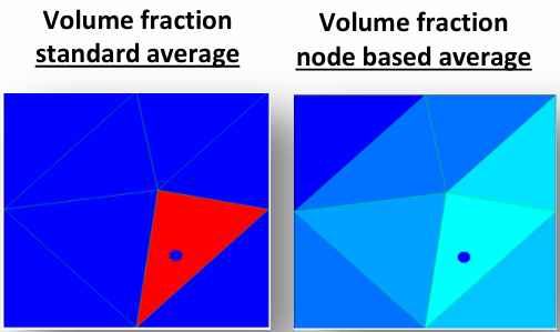
Figure 11: Always enable Node-Based Averaging in the DPM Numerics tab; it smoothly distributes the volume fraction to prevent the solver from crashing when parcels pack tightly.
Numerical Schemes for Multiphase Flows
In Eulerian multiphase simulations, the transport equations for the continuous fluid and the discrete solid phases are heavily linked through massive mathematical source terms. Because drag and collision forces create such extreme pressure gradients, solving these coupled equations requires advanced numerical algorithms. To manage this complex pressure-velocity coupling, ANSYS Fluent offers two primary mathematical schemes: Phase Coupled SIMPLE (PC-SIMPLE) and the Full Multiphase Coupled solver.
The PC-SIMPLE algorithm solves the secondary phase volume fractions in a completely segregated manner, meaning it solves one equation at a time to save RAM, but it is highly vulnerable to numerical divergence.
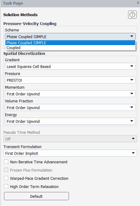
Figure 12: Engineers must carefully choose between the segregated PC-SIMPLE scheme or the robust Coupled scheme in the Solution Methods panel.
Multiphase Coupled Solver
To completely overcome the stability limitations of the segregated PC-SIMPLE approach, engineers highly recommend utilizing the Multiphase Coupled Solver. Instead of solving the physics step-by-step, this advanced algorithm simultaneously solves the volume fraction, pressure, and momentum equations in one massive unified matrix.
The Multiphase Coupled solver provides vastly superior robustness and efficiency for steady-state problems, easily powering through dense particle packing that would normally crash a segregated solver.
However, for transient simulations, the computing efficiency of the coupled solver decreases significantly if your continuous fluid time step is extremely small. To regain computational speed during transient runs, you must increase your fluid time steps to utilize the coupled solver’s full potential.
Conservative Solver Settings
If hardware memory limitations force you to use the PC-SIMPLE algorithm, starting your simulation with highly aggressive parameters will instantly crash the solver. You must establish strict, conservative mathematical settings to gently ease the fluid equations into stability.
If the volume fraction residuals oscillate or convergence remains incredibly slow, you must manually adjust the Multi-Grid and Under-Relaxation Factors (URFs) inside the Solution Controls panel. Here is a quick-guide table for configuring strict conservative settings in PC-SIMPLE:
| Solver Parameter | Mathematical Function | Recommended Setup in Fluent |
| Pressure Multi-Grid | Controls the mathematical grid coarsening used to solve pressure. | Lower it by two orders of magnitude (e.g., set to 0.001 instead of the default 0.1). |
| Volume Fraction URF | Limits how fast the phase boundaries can change per iteration. | Reduce safely down to a range of 0.2 to 0.5. |
| Velocity & Pressure URF | Stabilizes the continuous fluid flow field. | Swap them! Start conservatively at 0.3 for momentum and 0.7 for pressure. |
| Gradient Stabilization | Prevents artificial numerical spikes across sharp particle boundaries. | Strictly enable BCGSTAB to smooth out mathematical gradients. |
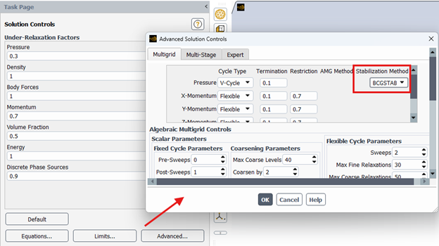
Figure 13: When using PC-SIMPLE, engineers must manually lower the Under-Relaxation Factors to heavily stabilize the volume fraction equations.
Conclusion
Learning Eulerian multiphase simulations in ANSYS Fluent requires a deep engineering understanding of interphase physics and strict numerical discipline. By carefully selecting the appropriate DDPM or DEM mathematical approach, accurately defining physical collision partners, and strictly controlling your fluid and particle time steps, you can achieve highly stable industrial simulations. Always prioritize clean mesh generation and conservative initial solver settings to guarantee successful particulate modeling, from fluidized beds to complex dense drying reactors!