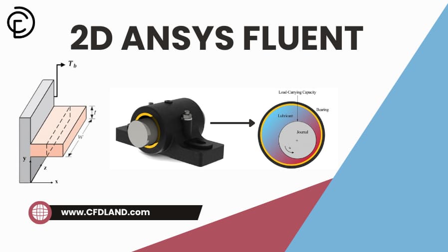
2D ANSYS Fluent Simulation: Step-by-Step 2D CFD Tutorial

2D ANSYS Fluent simulations offer an efficient way to study fluid flow and heat transfer when the third dimension is not significant. A 2d fluid dynamics simulation solves the flow on a single plane instead of a full volume. It runs in minutes instead of hours, and for many problems the answer is the same.

If your model’s geometry is uniform in the third dimension, especially along the z-axis (for instance), then an ansys 2d simulation setup is highly suitable. With benefits like faster computation, simpler meshing, and reduced hardware demand, they’re ideal for concept testing, education, and early-stage analysis. This blog is a comprehensive tutorial that walks you through the full simulation process—geometry,meshing, setup, solution, and post-processing. Common examples include flow over a cylinder, airfoil analysis, long, straight pipes and ducts, and axisymmetric problems. After reading this blog, you will be able to confidently set up and run your own Ansys 2d analysis from start to finish.

When to Use 2D ANSYS Fluent Simulations

While the real world is three-dimensional, opting for an Ansys fluent 2d simulation is often a smart and efficient choice under specific circumstances. Understanding when to leverage ANSYS Fluent 2D capabilities saves significant computational time without compromising essential engineering insights.

Geometric Uniformity along One Axis

If the geometry is very long in one dimension (extruded) and the flow characteristics do not change significantly along that length, a 2D cross-section accurately represents the behavior. Examples include flow over long airfoils, flow in wide channels, pipes, or heat transfer through uniform walls.

A classic example is the analysis of lubricant flow in a journal bearing, where the thin film of lubricant between the rotating journal and stationary bearing is modeled in two dimensions (Fig.1). This 2D analysis assumes a uniform distribution of pressure and oil film along the bearing’s axial direction. In other words, the flow is fully developed in the z-direction (bearing depth), meaning it can be approximated as infinitely long. This infinitely long approximation justifies using a 2D planar model instead of a full 3D simulation because variations along the bearing length are negligible.

              

Figure 1- (a) 3D journal bearing geometry  vs. (b) 2D journal bearing geometry  [1]

The Lift-Drag Optimization on Airfoil Using Mesh Morphing (RBF) offers a practical approach to enhancing aerodynamic performance by applying Radial Basis Function mesh morphing in a 2D airfoil simulation (Fig.2). This method allows for dynamic shape modifications without full domain remeshing, enabling efficient exploration of design alternatives. By combining RBF morphing with optimization algorithms, the tutorial focuses on improving the lift-to-drag ratio under specified flight conditions.

Figure 2- Lift-Drag optimization on 2D airfoil simulation using Mesh Morphing (RBF)

Axisymmetric Symmetry (2D Axisymmetric)

When the geometry and flow are symmetrical around a central axis, an Ansys fluent 2d axisymmetric model is highly effective (Fig.3). This applies to flow through pipes, nozzles, diffusers, around cones, or certain types of valves.

Figure 3- ANSYS Fluent 2d assumption

The Compressible Flow in Nozzle CFD Simulation demonstrates how axisymmetric behavior justifies the use of 2D models for analyzing high-speed compressible gas flow. This tutorial focuses on key characteristics—velocity, pressure, and temperature—within a nozzle.

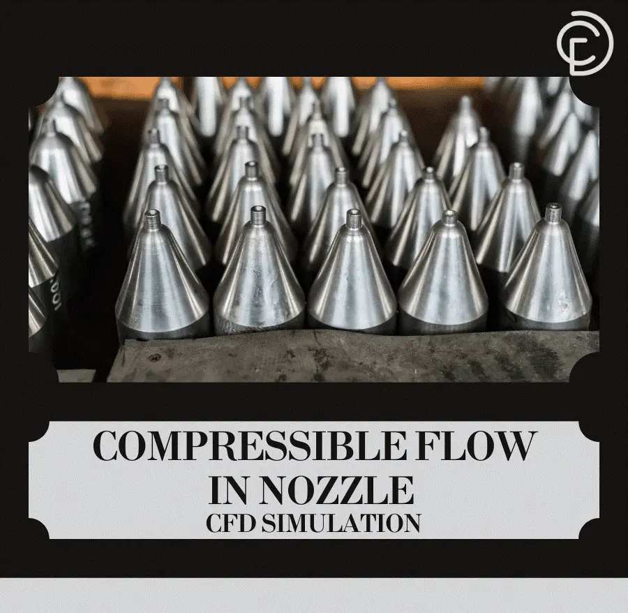
Figure 4- Compressible Flow in Nozzle CFD Simulation, ANSYS 2D axisymmetric analysis

Dominantly 2D Flow Behavior

The flow field should not vary significantly in the third direction. When velocity, pressure, or temperature gradients are negligible along the out-of-plane axis, a 2D analysis is optimal. For example, as shown in Fig.5, the fin extends far in the x-direction, and its thickness 𝑡 is very small compared to its length. Therefore, we can neglect any variation in the z-direction.

Figure 5- Long rectangular fin with dominantly 2D heat transfer behavior[3]

When Should You Avoid Using 2D in ANSYS Fluent?

While 2D simulations are efficient, there are important situations where relying on a 2D model leads to inaccurate results. Avoid 2D approximations when:

• Strong 3D Effects Exist: Swirling flows, secondary flows, or end effects require full spatial modeling.
• Geometry Is Not Uniform: If the geometry changes along the third dimension (e.g., bends, junctions), 2D simplifications are invalid.
• Transient 3D Phenomena: Flows involving turbulent eddies or vortex shedding that evolve in three dimensions require 3D modeling.
• Accurate Quantitative Predictions Needed: Final design validation or safety-critical applications demand comprehensive 3D results.

2D vs 3D CFD Simulation Comparison

Feature	2D Simulation	3D Simulation
Cell count	20k – 100k	1M – 10M+
Run time	Minutes	Hours to days
Hardware	Laptop	Workstation / cluster
Captures swirl & secondary flow	No	Yes
Best for	Concept testing, education, parametric studies	Final validation, certification
Typical cases	Airfoil, pipe, nozzle, journal bearing	Manifolds, bends, mixers, rotating machinery

The Flow Through A Pipe CFD Simulation focuses on validating analytical results from Cengel’s Fluid Mechanics. Modeled as Session 2 of the ANSYS Fluent Course for Beginners, it offers a clear comparison between CFD and textbook-based solutions for steady oil flow.

Figure 6- Flow through a pipe CFD simulation | ANSYS Fluent 2d pipe flow

 

Step-by-Step Guide to 2D Fluid Flow Modeling

Here, we provide a practical tutorial example of 2D fluid flow simulation, demonstrated through the flow around a cylinder. Fig.7 illustrates different flow regimes around a cylinder based on the Reynolds number.

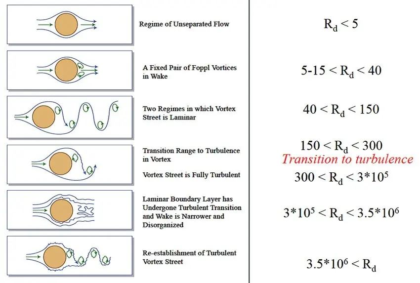
Figure 7- Formation of vortices for various Reynolds number[4]

Step1: Activating Fluid Flow (Fluent) Analysis System

After launching ANSYS Workbench, drag and drop the Fluid Flow (Fluent) analysis system from the Toolbox into the Project Schematic area (Fig.8).

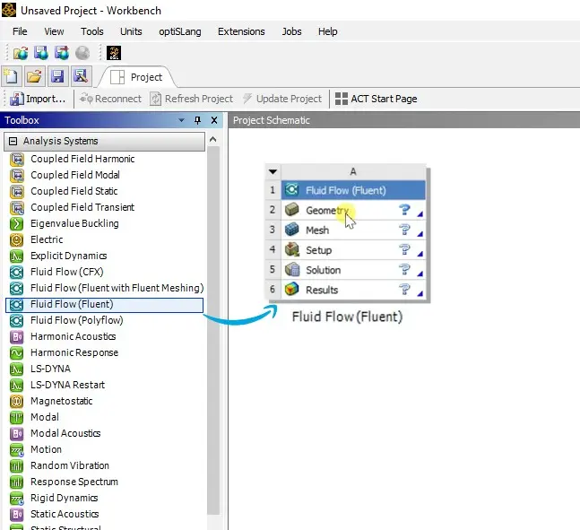
Figure 8- How to adding fluid flow (Fluent) system

Step2: Set Geometry Analysis Type to 2D

Click on the Geometry cell. In the Properties panel, find Advanced Geometry Options and set the Analysis Type to 2D. This configures the solver for a planar environment.

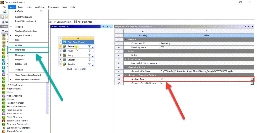
Figure 9- Setting geometry analysis type to 2D in ANSYS Workbench

Step3: Creating the Geometry

Preparing a domain for a 2d CFD simulation is slightly different from 3D. If starting with a 3D CAD model, extract a mid-plane slice to act as your 2D sketch. ANSYS requires this sketch to be a fully closed surface (a surface body), not just wireframe edges.

For external flow over a cylinder, position the object inside a rectangular boundary. Extend the domain roughly 10 to 20 diameters downstream. This extra space allows the turbulent wake to develop fully without hitting the pressure outlet boundary prematurely, ensuring physical accuracy.

Figure 10- Schematic Diagram of the 2D Flow Domain Showing Boundary Conditions and Cylinder Position[5]

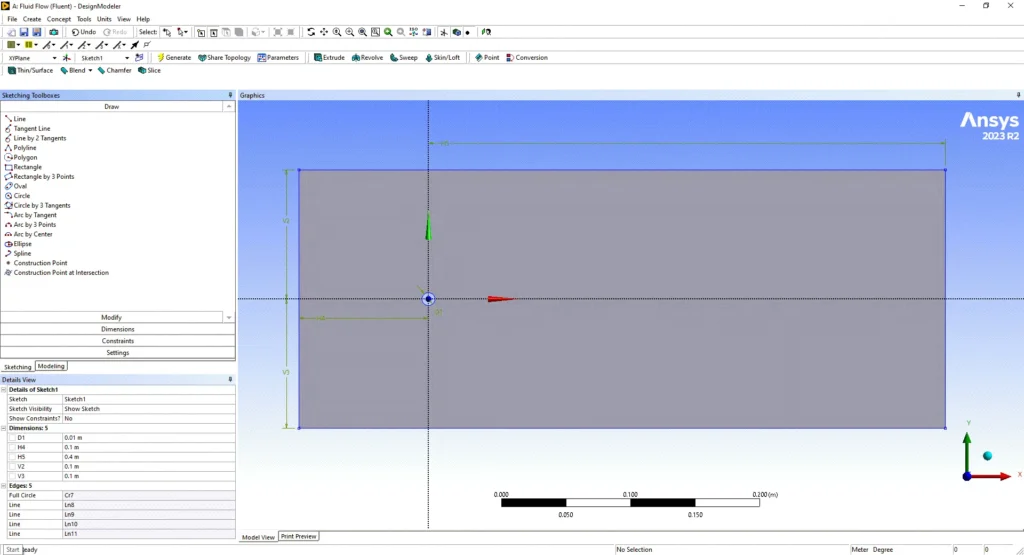
Figure 11- Geometry Setup of the 2D Flow Domain with Cylinder in ANSYS DesignModeler

Step 4: 2D Meshing in ANSYS Fluent

A common point of confusion for beginners is finding the correct tool for fluent meshing 2d operations. The modern ANSYS Fluent Meshing interface (which features watertight and mosaic workflows) is built exclusively for 3D volumes.

To perform Ansys fluent 2d meshing, use the standard ANSYS Meshing module or DesignModeler. In a 2D space, mesh types in CFD are restricted to quad (quadrilateral) and tri (triangular) elements. A structured quad mesh is highly recommended for 2D planar flows because it aligns better with the flow direction and reduces numerical diffusion.

For the flow over a cylinder, apply inflation layers around the cylinder wall. This creates a dense grid of prism layers near the surface, allowing the solver to accurately capture the boundary layer and maintain the correct y+ value. Additionally, use edge sizing with a bias toward the cylinder to capture the immediate wake. Because a 2D domain ignores volume, a typical cell count ranges from just 20,000 to 100,000 cells. To fully master these grid controls, refer to our comprehensive FREE ANSYS MESHING COURSE.

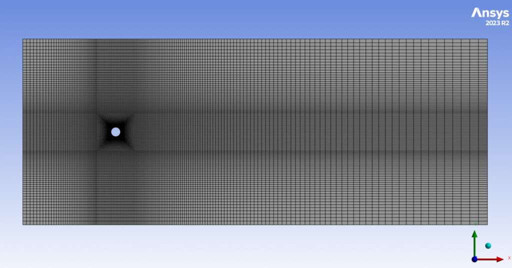
Figure 12- mesh generation for 2d flow domain around a cylinder

Step 5: Defining Named Selections

Clearly identify and label the boundaries where different flow conditions apply. Create four named selections: “inlet” (left), “outlet” (right), “cyl-wall” (cylinder surface as a no-slip wall), and “symmetry” (top and bottom).

The next step is to define the boundary conditions by creating named selections for different parts of the geometry (Fig.13). In ANSYS Fluent meshing, you need to clearly identify and label the boundaries where different flow conditions will be applied. Here, four named selections are created: “inlet” on the left side where the fluid enters the domain, “outlet” on the right side where the fluid leaves, “cyl-wall” which represents the surface of the cylinder as a no-slip wall, and “symmetry” on the top and bottom boundaries to assume symmetric flow and reduce computational effort.  These named selections help you assign the correct boundary conditions later in the fluent solver setup, ensuring the simulation accurately represents the physical problem.

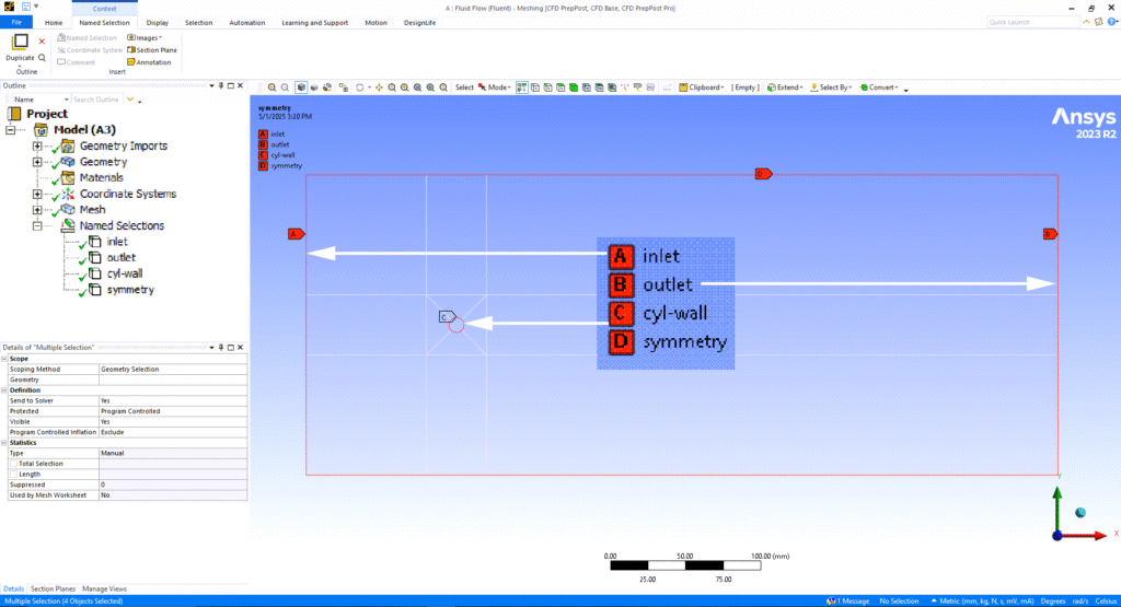
Figure 13- Boundary conditions and named selections setup for 2d flow around a cylinder in ANSYS Fluent

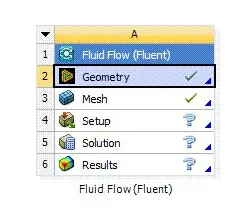
Figure 14- Simulation workflow progress in ANSYS Fluent

Step 6: Fluent Launcher and 2D Space

Open the setup cell to access the Fluent Launcher. The dimension defaults to 2D based on your geometry settings. Enable double precision to ensure higher numerical accuracy during matrix calculations. Under the General task page, check the 2D Space settings. For standard flat simulations, select “Planar.” If the geometry rotates around a central axis, select “Axisymmetric.”

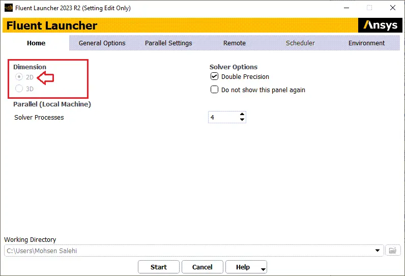
Figure 15- Fluent launcher setup window for selecting simulation dimension and solver options

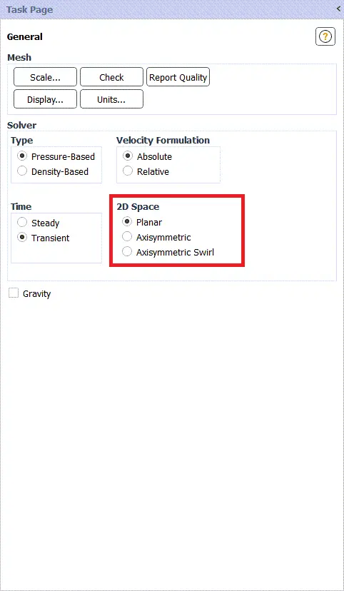
Figure 16- Task page for defining solver settings and 2d space geometry type

Step 7: Selecting the Viscous Model

Navigate to the Models tree. For flow at Re ≈ 10,000, the boundary layer is still laminar, but the wake is turbulent and sheds vortices periodically (the subcritical regime). Select the k-ω SST turbulence model to accurately capture flow separation and wake dynamics.

Step 8: Defining the Material

Under Materials, edit the fluid properties (density and viscosity) to match your target Reynolds number. For this tutorial, standard air properties are suitable, provided the inlet velocity scales correctly to Re=10,000.

Step 9: Applying Boundary Conditions

Assign the physical values to the named selections from Step 5. Set the inlet to a “Velocity-Inlet” with a specified speed. Leave the outlet as a “Pressure-Outlet” at zero gauge pressure. The cylinder defaults to a stationary “Wall.”

Step 10: Solution Methods and Initialization

In the Solution Methods panel, select the SIMPLE or Coupled scheme with second-order upwind spatial discretization. Proceed to Initialization and select “Hybrid Initialization” to provide the solver with a stable starting pressure field.

Step 11: Running the Calculation

Specify the number of iterations and start the calculation. Relying solely on residuals can be misleading. Always create a report definition to monitor the drag coefficient on the cylinder to judge physical convergence, as outlined in our ANSYS Fluent Convergence guide.

Step 12: Reference Values

Finally, verify the Reference Values section. Set “Compute from” to the inlet. The solver uses these reference values (area, density, velocity) to accurately calculate dimensionless coefficients like lift and drag during post-processing.

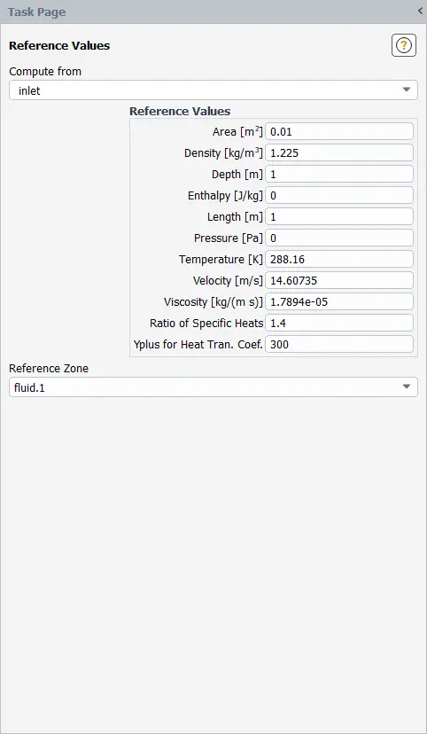
Figure 17- Reference values panel in ANSYS Fluent

Step 13: Post-Processing the 2D Flow Results

Fig. 18 shows a velocity contour plot generated in ANSYS Fluent’s post-processing tool. The color map represents the velocity magnitude, highlighting flow behavior as it interacts with the cylinder. The flow separates at the surface, forming a recirculation wake behind it, which is typical for this Reynolds number (Re ≈ 10,000). The wake features low velocities, while the fluid accelerates further downstream.

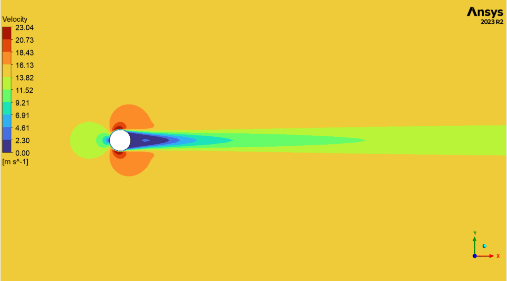
Figure 18- Velocity contour plot around a cylinder in a 2D flow simulation

The Unsteady Vortex Shedding behind Cylinder CFD Simulation explores this exact phenomena further. It demonstrates key 2d CFD flow behaviors such as boundary layer separation, wake formation, and the von Kármán vortex street. Widely used in engineering, this case helps analyze vortex-induced vibrations affecting structures like bridges and towers.

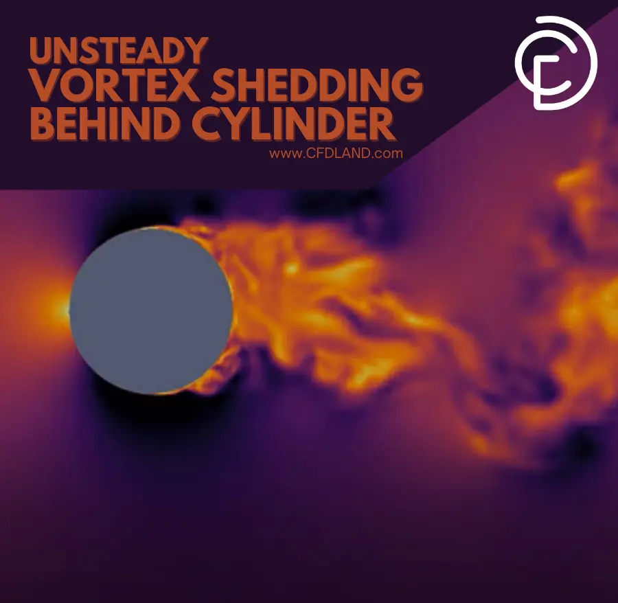
Figure 19- Unsteady vortex shedding behind cylinder CFD Simulation, ANSYS Fluent 2d tutorial

Conclusion

2D ANSYS Fluent simulations provide a highly efficient way to analyze fluid dynamics when the third dimension is negligible. By leveraging geometric uniformity and axisymmetric boundaries, these simulations deliver reliable results with reduced hardware costs and faster processing times. This tutorial serves as a baseline guide, enabling engineers to confidently set up their own models and gain a deeper understanding of computational fluid dynamics.

You can practice with our free CFD simulation trainings before running your own 2D case. If you need a 2D or 3D CFD case run on your own geometry, you can order a CFD project.

 

FAQs

• Can you use ANSYS Fluent Meshing for a 2D model? No. ANSYS Fluent Meshing and its automated watertight workflows are built exclusively for 3D geometries. To mesh a 2D domain, use the standard ANSYS Meshing module or DesignModeler and ensure your geometry is set to a 2D analysis type.
• What is the difference between planar and axisymmetric in ANSYS Fluent 2D? A planar model solves flow across a flat 2D slice with a uniform depth. An axisymmetric model revolves a 2D profile around a central axis, effectively simulating a full 3D cylindrical volume (like a pipe or nozzle) using only a 2D plane.
• How do I convert a 3D geometry to a 2D model in ANSYS? Extract a mid-plane slice from your 3D CAD model. Ensure this slice is a closed surface body, not just wireframe lines. When importing this surface into ANSYS Workbench, change the Geometry Analysis Type in the properties panel to 2D.
• Is a 2D CFD simulation accurate? Yes, a 2D simulation is highly accurate provided the physical flow lacks strong three-dimensional effects. If there are no cross-stream vortices, spanwise gradients, or 3D geometry changes, a 2D solver produces identical results to a 3D solver in a fraction of the time.

 

Reference

[1]        A. Abbaspur et al., “An analytical study on nonlinear viscoelastic lubrication in journal bearings,” Scientific Reports, vol. 13, no. 1, p. 16836, 2023.

[2]        H. Zhang, J. Li, H. Li, H. Ye, H. Zhang, and Y. Zheng, “A coupled axisymmetric peridynamics with correspondence material model for thermoplastic and ductile fracture problems,” International Journal of Fracture, vol. 244, no. 1, pp. 85-111, 2023.

[3]        T. L. Bergman, Fundamentals of heat and mass transfer. John Wiley & Sons, 2011.

[4]        A. P. Pandey, A. Sawla, S. Kr Gupta, and P. Baredar, “VIVEC (Vortex Induced Vibration Energy Converter): A new and renewable approach to harness the hydro-kinetic energy of geophysical fluid flow,” International Journal Of Advance Research In Science And Engineering, vol. 5, pp. 1-20, 2016.

[5]        S. Ye, Z. Zhang, X. Song, Y. Wang, Y. Chen, and C. Huang, “A flow feature detection method for modeling pressure distribution around a cylinder in non-uniform flows by using a convolutional neural network,” Scientific reports, vol. 10, no. 1, p. 4459, 2020.