ANSYS Fluent Expressions: Syntax, Functions and Examples

Have you ever wondered how to get rid of writing User-Defined Functions (UDFs) in ANSYS Fluent? The good news is that starting from ANSYS 2019 R1, a powerful and exciting feature called the Fluent Expression Language was introduced to make that possible.

In the past, even simple tasks like setting a boundary condition required writing UDFs in C programming language, dealing with unit conversions, and learning Fluent-specific programming. But now, with Ansys fluent expressions, you can define logic, formulas, and custom conditions directly in the User Interface (UI) without writing a single line of code (Fig.1). This study covers everything from using the expression editor, an example, writing IF conditions, understanding syntax, fixing errors like “expression is not single valued,” to applying report definitions and working with named expressions.

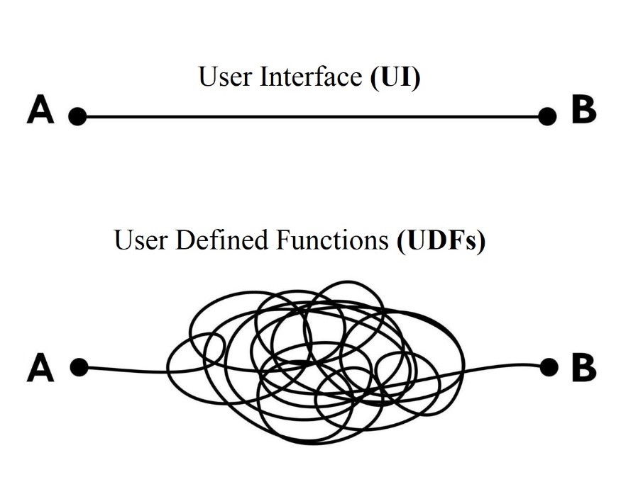
Figure 1- How Expressions in ANSYS Fluent Simplify Our Work

Expressions in ANSYS Fluent 

In CFD simulations, there are situations where boundary conditions, source terms, material properties, and other key parameters need to be defined as nonuniform mathematical functions of time or space. These functions may depend on variables from different locations or other aspects of the solution. In ANSYS Fluent, such complex dependencies can be handled using a fluent expression.

ANSYS Fluent User Interface (UI) allows users to customize and organize simulation workflows, define new variables for post-processing, enable parametric studies, and more. For instance, Fig.2 shows you the Fluent UDF code required to set up a sinusoidally fluctuating heat source based on the function Energy(t) = 90000*sin(t) [W/m^3].

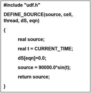
Figure 2- Defining a sinusoidally fluctuating heat source based on the function via UDF code

Even a simple UDF, like the one in Fig.2, requires significant effort, including unit conversion, C programming, and learning Fluent-specific concepts. This can be time-consuming even for experienced users. Fluent UI expressions simplify this by allowing users to enhance simulations without writing or compiling UDFs (Fig.3). They enable the use of mathematical functions, logical operators, and fluent field variables to define complex boundary and cell zone conditions more easily.

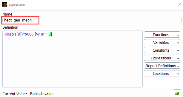
Figure 3- Defining a sinusoidally fluctuating heat source based on the UI expressions

User Interface (UI) Expressions vs. User-Defined Functions (UDFs)

Overall, UI Expressions are ideal for users looking for quick, straightforward solutions without extensive coding knowledge. They simplify workflows and improve productivity for most common simulation tasks. On the other hand, UDFs are better suited for advanced users who need complete control and customization over their simulations, especially for highly specialized or computationally demanding scenarios. Table 1 shows a comparison between UI and UDF in ANSYS Fluent.

Table 1- Comparison between UI and UDFs in ANSYS Fluent

Feature	User Interface (UI)	User-Defined Functions (UDFs)
Ease of Use	Easy to use, no coding required	Requires programming skills (usually in C)
Flexibility	Suitable for common tasks and conditions	Highly customizable for complex scenarios
Setup Time	Quick setup using graphical interface	Time-consuming due to coding, compiling, and debugging
Learning Curve	Low – suitable for beginners	Steep – suitable for advanced users
Applications	Ideal for simple to moderately complex conditions and post-processing tasks.	Best for handling highly specialized or unconventional simulation scenarios.

When an expression is not enough, the next step is code, explained in our guide to ANSYS Fluent UDF.

Applications

If you’re looking for a practical example to learn how to use expressions in ANSYS Fluent, CFD LAND provides a tutorial for this purpose. In “CuO Nanofluid Effect on Cooling Performance Considering Thermal Resistance CFD Simulation, Numerical Paper Validation”, Fluent Expressions are used to calculate thermal resistance, while the UI streamlines setup and analysis. This case shows how CuO nanofluids enhance heat transfer for efficient cooling system design (Fig.4).

Figure 4- CuO Nanofluid Effect on Cooling Performance Considering Thermal Resistance, Numerical Paper Validation

Moreover, CFDLAND provides another tutorial for learning how to use expressions in thermal boundary conditions, applied in a real industrial context. The training “Steam Methane Reforming (SMR) Reaction CFD Simulation (2D) – Numerical Paper Validation” focuses on simulating a highly endothermic reaction used for hydrogen production. Since the reaction kinetics do not follow the standard Arrhenius model, a UDF was written to define the custom behavior. Additionally, a temperature gradient at the upper wall—as described in the reference paper—is implemented using an expression in Fluent, making this a valuable example of combining physical accuracy with Fluent’s expression capabilities (Fig.5).

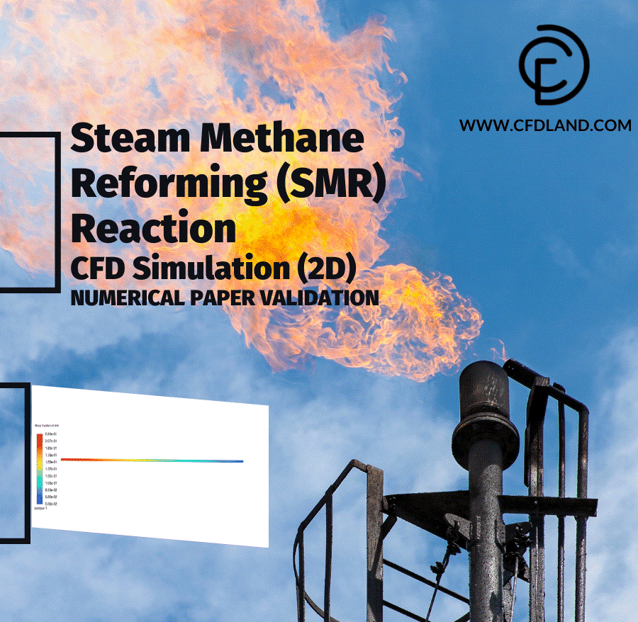
Figure 5- Steam Methane Reforming (SMR) Reaction CFD Simulation (2D) – Numerical Paper Validation

What You Need to Know Before Writing Expressions

To effectively learn and use the ANSYS Fluent User Interface (UI), it is essential to have a foundational understanding of the Expression Syntax and the types of variables, such as Field Variables (e.g., velocity, temperature) and Solution Variables (e.g., pressure gradients, turbulence parameters). Additionally, knowledge of Scientific Constants (e.g., thermal conductivity, specific heat) and the use of Aliases for simplifying complex expressions is crucial. Understanding the methods for applying expressions—whether through boundary conditions, cell zone conditions, or post-processing tasks—is equally important to streamline workflows effectively. Beyond these, familiarity with the ANSYS Fluent environment, and an ability to navigate tools like the Expression Editor and Report Definitions will enhance your ability to define and manage expressions efficiently. Following this, we will explore step by step all of the necessary things you should know about ANSYS Fluent User Interface (UI) expressions.

 

Fluent Expression Syntax

An expression is a string that represents a combination of: Values, Variables, Operators and Function calls. When an expression is evaluated with appropriate values assigned to its variables, it returns a resulting value (which can be a Number, Boolean, or Field). Grasping correct fluent expression syntax prevents solver errors.

Fluent Expression Syntax Rules

To write formulas successfully, follow these strict Ansys expression syntax rules:

1. Units always go inside square brackets (e.g., [m/s], [Pa]).
2. Names are case-sensitive (Time is different from time).
3. Variable names cannot start with a number.
4. Do not chain comparison operators (use AND() instead of 400[K] > T > 300[K]).
5. Context requires explicit naming (e.g., species="co2").
6. Standard math hierarchy applies (parentheses resolve first).
7. Position relies on standard aliases (x, y, z).

Expression Data Types

The evaluated result of an expression can be a real number, a Boolean, a real field or a Boolean field. Table 2 depicts types of expression data.

Table 2-Expression Data Types

Type	Description
Real Number	A scalar value like 3.14 or -1.0e-3
Boolean	Logical value: true or false
Real Field	2 * StaticPressure
Real Single Values	average(2*StaticPressure, [“inlet”])

Operators

Here’s a full summary of common Operators used in ANSYS Fluent expressions (Table 3).

Table 3- Common Operators used for expressions writing

Operator	Function
+, -, *, /	Basic arithmetic
**	Power
<, <=, >, >=, ==, !=	Comparisons

❗ Important: Do not chain comparison operators directly. Use logical functions instead, e.g.

AND (StaticTemperature > 300[K], StaticTemperature < 400[K]) ✅

400[K] > StaticTemperature > 300[K] ❌

Mathematical and Logical Functions

Mathematical and logical functions (Table 5) perform basic operations like absolute value, exponentiation, logarithms, etc. The complete Ansys expression list provides deep flexibility for modeling.

Table 4-Common Mathematical and Logical ANSYS expression list

Function	Description
abs(<expr>)	Absolute value
exp(<expr>)	Exponential
log(<expr>)	Natural logarithm
log10(<expr>)	Base-10 logarithm
sqrt(<expr>)	Square root
round(<expr>)	Round to nearest integer
ceil(<expr>)	Ceiling (round up)
floor(<expr>)	Floor (round down)
trunc(<expr>)	Truncate
mod(a, b)	Modulus
max(a, b)	Maximum
min(a, b)	Minimum
sin(<expr>)	Sine
cos(<expr>)	Cosine
tan(<expr>)	Tangent
asin(<expr>)	Inverse sine
acos(<expr>)	Inverse cosine
atan(<expr>)	Inverse tangent
atan2(<expr1>, <expr2>)	Arctangent of (<expr1>)/(<expr2>)
sinh(<expr>)	Hyperbolic sine
cosh(<expr>)	Hyperbolic cosine
tanh(<expr>)	Hyperbolic tangent
asinh(<expr>)	Inverse hyperbolic sine
acosh(<expr>)	Inverse hyperbolic cosine
atanh(<expr>)	Inverse hyperbolic tangent

Logical and Conditional Functions in ANSYS are used to perform decision-based operations within expressions, allowing users to apply conditions (like IF, AND, OR) to control the outcome based on logical comparisons. These functions return either boolean values or numeric results depending on the condition, and are essential for region selection, conditional assignments, and adaptive modeling (Table 6).

Table 5- Logical and Conditional Functions Used in ANSYS Expressions

Function	Description
IF(cond, true_val, false_val)	If cond is true, returns true_val, else false_val
AND(expr1, expr2, …)	Logical AND
OR(expr1, expr2, …)	Logical OR
XOR(expr1, expr2)	Exclusive OR
NOT(expr)	Logical negation

Reduction Functions

Reduction Functions in ANSYS (Table 6) compute summary values—such as average, maximum, minimum, sum, area, or volume—over specified regions or zones in the computational domain. They help extract global or regional insights from field data.

Table 6- Reduction Functions in ANSYS Expression Syntax

Function	Description
Area([loc])	Returns the area of a region
Volume([loc])	Returns the volume of a region
Average(expr, [loc])	Average of the expression over the region
Maximum(expr, [loc])	Maximum value over specified region
Minimum(expr, [loc])	Minimum value over specified region
Sum(expr, [loc])	Total of the expression over a region
MassFlowAve(expr, [loc])	Mass-flow weighted average
MassFlowInt(expr, [loc])	Mass-flow integral
AreaAve(expr, [loc])	Area-weighted average
AreaInt(expr, [loc])	Area integral
MassAve(expr, [loc])	Mass-weighted average
FlowRate([loc])	Mass or volume flow rate

Vector Operations

Vector Operations in ANSYS (Table 7) allow users to access specific components (x, y, z) or the magnitude of a vector field such as velocity or force, enabling detailed directional analysis and calculations.

Table 7- Vector Operations in ANSYS Expressions

Syntax	Description
Velocity.x	x-component of the vector
Velocity.y	y-component of the vector
Velocity.z	z-component of the vector
Velocity.mag	Magnitude of the vector

Field Variables in ANSYS Fluent

In ANSYS Fluent, field variables refer to physical quantities that vary across the computational domain—such as velocity, pressure, temperature, species concentration, etc. These variables are essential for postprocessing and can also be used directly in expressions to define custom functions, conditions, or field-dependent inputs. Some variables require additional context, which is specified in the following format: Variable (<context>=”<context value>”).

• To get the species mass fraction of carbon dioxide. For example:

MassFraction (species=”co2″)

• In multiphase simulations, the phase context must be specified. For example:

MassFraction (species=”co2″, phase=”air”)

Important Notes:

1. Context must be explicitly specified using named parameters like species, phase, or mixture.
2. Variables like pressure, temperature, and velocity typically do not require context.
3. Multiphase simulations (VOF, Eulerian, etc.) must include the phase context when accessing phase-specific properties.

 

Solution Variables in Fluent

Solution variables are global simulation values representing time, iteration, or timestep-related information (Table 8). These are accessible during the simulation and can be referenced in custom expressions, conditionals, or user-defined operations.

Table 8- Available Solution Variables in ANSYS Fluent

Variable	Description
Time	Returns the current simulation time. In steady-state, it evaluates as 0, unless the case was previously run as transient, in which case it retains the last transient time.
Timestep	Returns the current timestep number. Same as above — 0 in steady-state unless switched from transient.
DeltaTime	Returns the time step size used in the current iteration. Again, 0 in pure steady-state unless continued from transient.
Iteration	Returns the global iteration count (i.e., how many solver iterations have occurred).

Important Notes:

• In steady-state simulations, Time, Timestep, and DeltaTime will return 0 unless the simulation was previously run in transient mode and then switched to steady. These variables are especially useful for:

• Creating time-dependent expressions (e.g., oscillating sources).
• Triggering changes based on iteration number.
• Controlling time-based boundary conditions or sources.

 

Scientific Constants

Scientific constants are predefined physical values like π, e, the gas constant ®, and gravitational acceleration (g) that are universally accepted in scientific and engineering calculations. Table 10 provides comprehensive scientific constants important in writing ANSYS Fluent expressions.

Table 9- Fundamental Scientific Constants

Variable	Description	Value
PI	Pi	3.14159265358979323846
e	e (base of the natural logarithm)	2.71828182845904523536
R	Gas constant	8.314472 [J K^-1 mol^-1]
avogadro	Avogadro’s number	6.02214199e23 [mol^-1]
boltzmann	Boltzmann constant	1.3806503 [J K^-1]
clight	Light velocity	2.99792458e8 [m s^-1]
echarge	Electron charge	1.60217653e-19 [A s]
g	Acceleration due to gravity	9.8066502 [m s^-2]
planck	Planck’s constant	6.62606876e-34 [J s]
stephan	Stefan-Boltzmann constant	5.670400e-08 [W m^-2 K^-2]
mupermo	Magnetic permeability of free space	4.0*PI*1.0e-7 [N A^-2]
epspermo	Electric constant	1./(clight*clight*mupermo)

Aliases

Aliases provide simplified syntax to access frequently used variables (Table 10).

Table 10- Types of available variable in ANSYS Fluent and the corresponding Aliases

Variable	Alias to
x	Position.x
y	Position.y
z	Position.z
u	Velocity.x
v	Velocity.y
w	Velocity.z
iter	Global iteration count
T	StaticTemperature
P	StaticPressure
mf	MassFraction
Amag	FaceAreaMagnitude
vol	CellVolume
mass	CellVolume*Density
t	Time*
dt	DeltaTime**

Important Notes:

• *In steady state, time (t) evaluates as 0, unless the case was run in transient, then switched to steady state, in which case it will evaluate as the latest time from the transient run.
• **In steady state, delta time (dt) evaluates as 0, unless the case was run in transient, then switched to steady state, in which case it will evaluate as the latest delta time from the transient run.

Using IF Conditions in Fluent Expressions

An Ansys fluent expression if statement creates dynamic boundaries or time-triggered events. The syntax follows this structure: IF(Condition, Value_if_True, Value_if_False).

For a time-triggered switch, like a valve opening after 2 seconds, apply this to a velocity inlet: IF(Time > 2 [s], 5 [m/s], 0 [m/s])

For a temperature-dependent source, like a heater activating when the local cell temperature drops below 300 K, apply this to the cell zone energy source: IF(StaticTemperature < 300 [K], 1000 [W/m^3], 0 [W/m^3])

 

Expressions vs Custom Field Functions

Before modern expressions existed, users relied on the fluent custom field function tool to create new variables for post-processing. You access this older tool via Results → Custom Field Functions. While still functional, modern UI expressions are faster and replace this workflow entirely. For example, to plot a custom scalar based on absolute pressure, writing an expression in the Named Expressions panel is much quicker than using the old Custom Field Function calculator.

Using Expressions in Report Definitions

Expressions become highly powerful when combined with Report Definitions. Rather than exporting raw data, create a custom output monitor. For example, to track the mass-averaged temperature at an outlet, write an expression using the massflowave function: MassFlowAve(StaticTemperature, ["outlet"]). Assign this expression directly into a Report Definition to plot it live during the run.

Common Expression Errors

Expression errors behave like most solver messages, and the wider list is in our guide to common ANSYS Fluent errors.

• “Expression is not single valued”: This occurs when a field variable (varying across cells) is placed into a box requiring a single scalar number (like a mass flow rate input). Fix this by wrapping the variable in a reduction function like Average().
• Missing Units: If a velocity is multiplied by time to get a distance, the solver expects the final unit to be meters. Forgetting to specify [s] for time triggers a unit mismatch error.
• Missing Context: Calling MassFraction in a multi-species run causes an error unless the context is explicitly stated, such as (species="air").

CFD-Post Expressions Note

Note that a cfd-post expression uses a different syntax from Fluent UI expressions. For instance, Fluent uses Velocity.mag, while CFD-Post requires Velocity.Magnitude. CFD-Post uses its own expression syntax, covered in our free CFD-Post course.

How to Use Expressions in ANSYS Fluent

There are two primary methods for creating and using expressions in the software:

Direct Input

Direct Input is quick and convenient for one-time use. In this method, you can write the expression directly in the required field (e.g., boundary condition, source term, monitor, etc.). Here, as an example, you will see step by step how to define an expression for a boundary condition.

Step1: Selecting the Boundary Conditions (here, the target B.C. is Velocity inlet)

To navigate to field variables in ANSYS Fluent, go to Setup in the Outline View, select Boundary Conditions, and choose the desired boundary (e.g., Inlet) (Fig.6). In the Task Page, under the appropriate tab (e.g., Momentum), you can define variables like Velocity Magnitude using predefined values or expressions by clicking the function icon (f(x)).

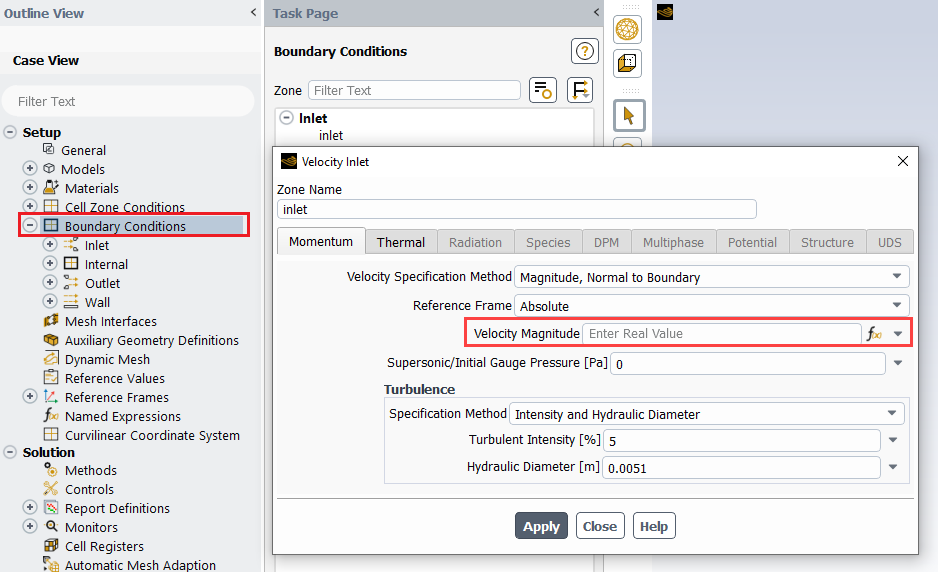
Figure 6- Navigation in ANSYS Fluent to Select Velocity Magnitude at an Inlet Boundary

Step2: Selecting the ANSYS Fluent expressions for setting the Boundary Condition

Click the drop-down arrow to the right of the field that you would like to define using an expression and select expression (Fig.7). Now, you can enter your expression directly in the text field. For example, Fig. 8 illustrates how you can set Velocity Inlet boundary condition via in ANSYS Fluent expressions.

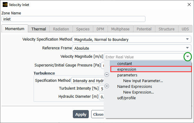
Figure 7- How to enable expressions for setting the Boundary Condition

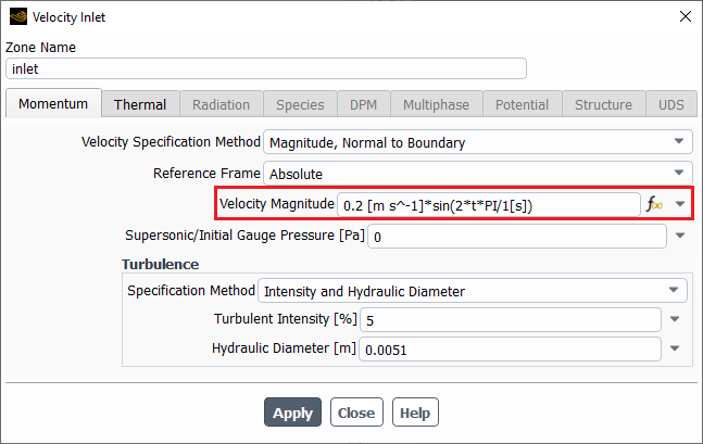
Figure 8- Setting the aim Boundary Condition within the expression editor Dialog Box

As shown in the Fig.8, the Velocity Magnitude is defined using a time-dependent function, and The Reference Frame is set to Absolute:

Velocity Magnitude= 0.2 [m/s] * sin (2 * t * π / 1[s])

• The velocity magnitude is defined as a sinusoidal function of time.
• 2 [m s^-1] is the amplitude of the velocity.
• sin(2*t*π/1 [s]) represents a sine wave with a frequency of 1 Hz.
• [m s^-1] specifies the velocity unit.
• [s] indicates the time unit.

Named Expression (Indirect Input)

Creating a Named Expression separately using the Expressions panel, allows you to assign a name to the expression and reuse it in multiple locations throughout the model, ensuring consistency and ease of updates. Referring back to Fig. 3, this example demonstrates step by step how to define it as an expression function.

Step1: Creating a Named Expression for Reuse in ANSYS Fluent

Firstly, go to Setup and expand the Named Expressions section. Right-click on it and select New to create a new expression (Fig.9).

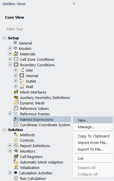
Figure 9- Navigation in ANSYS Fluent for Creating a new named expressions

Step2: Defining and Saving a Named Expression in ANSYS Fluent

Next, you should define the Named Expression by entering a name (e.g., heat_gen_mean) and specifying its mathematical formula or definition. You can use functions, variables, constants, or other expressions to build the definition. Once created, this expression can be reused in various parts of the simulation, then click OK to save it. Fig.10 shows a sinusoidally fluctuating heat source based on the time function:

Name = sin(t/1[s])*90000 [W/m^-3]

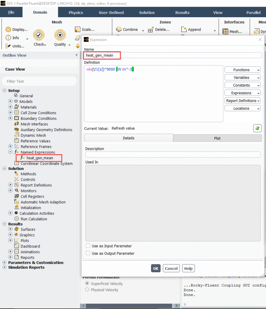
Figure 10- Defining and Saving a Named Expression in ANSYS Fluent

Step3: Using the Named Expression in a Boundary or Cell Zone

In Step 3, apply the created Named Expression in relevant simulation settings (here is stator). Then in the Cell Zone Conditions panel, navigate to the Source Terms, and for parameters like Energy Source, select Named Expressions from the dropdown (Fig.11).

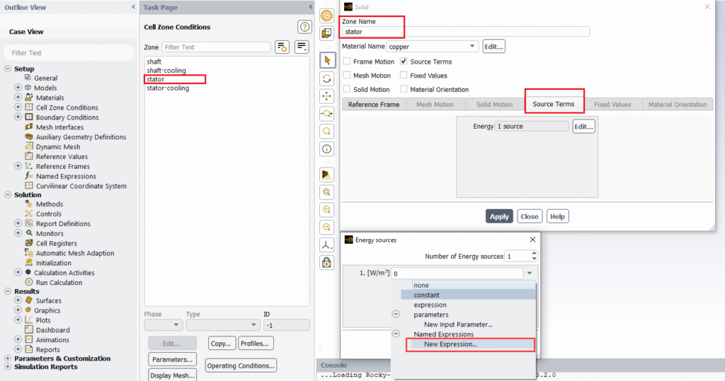
Figure 11- How to enabling the Named Expression, which is defined before, for a Boundary or Cell Zone

Step4: Activating the desired expression

Choose the desired expression, and click OK to use it in the simulation (Fig.12).

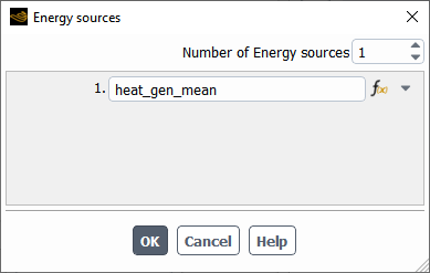
Figure 12- Activating the desired expression for keeping the simulation procedure

Context Specification

Some variables require additional context before they can be evaluated. For example, MassFraction requires the species context. Velocity may require phase context when it is evaluated in a multiphase simulation. The context is specified as a keyword argument to a function call on the variable. For example, MassFraction(species=”co2″, phase=”smoke”).

Supported Field Variables

In ANSYS Fluent, field variables represent physical quantities that can be accessed or manipulated during a simulation. These variables are essential for defining boundary conditions, post-processing, or writing custom User-Defined Functions (UDFs). Below you can see some examples of the field variables shown in the Table 12. It should be noted that ANSYS Fluent expressions supports a wide range of Field Variables; therefore, user can search for and utilize the specific variables needed for their simulations.

Table 12- Example of Field Variables suported in ANSYS Fluent

Description	Variable (type/context)
Absolute Pressure	AbsolutePressure (scalar)
Absolute Radiation Flux	AbsoluteRadiationFlux (scalar)
Axial Velocity	Axial Velocity AxialVelocity (scalar)
Cell Weight	CellWeight (scalar)
Density	Density (scalar)
Mass fraction of %s	MassFraction (species=”<species>”)
Dynamic Pressure	DynamicPressure (scalar)

For instance, Absolute Pressure (AbsolutePressure (scalar)), Represents the total pressure at a given point in the domain, including static and dynamic components. It is a scalar value commonly used for pressure-based calculations, boundary conditions, or monitoring.

Conclusion

The Expression Language simplifies CFD simulation setups by replacing complex C programming with intuitive formulas. Using the editor, engineers easily define time-dependent boundary conditions, dynamic source terms, and custom logical controls directly in the UI. Named expressions keep setups organized for parametric studies. Ultimately, leveraging these tools improves workflow efficiency, reduces coding errors, and streamlines data extraction.

FAQs

• What is the ANSYS Fluent Expression Language? It is a built-in feature that lets users define custom logic, formulas, and conditions directly in Fluent without writing UDFs.
• How do I enable expressions in ANSYS Fluent? Knowing how to enable expressions in ansys fluent is straightforward: click the f(x) icon next to input fields (e.g., velocity or energy), then select “Expression” to enter your formula.
• What is a good fluent expression example? A common fluent expression example is defining a time-varying parabolic velocity inlet, or setting a heat source that turns off when a specific temperature is reached using logical conditions.
• What is the difference between direct input and named expressions? Direct input is used for one-time expressions, while named expressions are reusable and created via the ANSYS Fluent expression editor.
• Can Fluent expressions replace UDFs? Yes, for many standard tasks like time-varying boundary conditions or logical controls. UDFs are still needed for advanced or highly customized behavior.