ANSYS Acoustic Models in Fluent: FWH, Broadband & Wave Equation

Welcome to our guide on ANSYS acoustic models. In our previous theory article, we learn the fundamental physics of sound. (If you need to review the basic physics, read our guide on what is aeroacoustics.)

Now, it is time to move from theory to practice. We will learn how to set up the ANSYS Fluent aeroacoustics tools, including:

• The Ffowcs-Williams & Hawkings (FWH) model
• Broadband Noise Source models
• The Wave Equation model

This practical guide shows you the main panels and essential settings for your CFD setup. A critical difference between these models is the solver requirement. For example, the FWH model uses an acoustic analogy that needs time-varying pressure data. Therefore, it always requires a transient solver. In contrast, the broadband noise source models use statistical methods to get noise data from a steady-state flow solution. This makes them much faster and perfect for early design comparisons.

To begin your setup, you can find all these tools in one central location. Navigate to: Problem Setup → Models → Acoustics.

Figure 1: Visualizing the acoustic noise distribution around a Horizontal-Axis Wind Turbine (HAWT). This is a common application for ANSYS acoustic models.

 

The Ffowcs Williams & Hawkings (FWH) Model

Many engineers ask: what is FWH? The Ffowcs Williams & Hawkings (FWH) model is the most widely used tool in ANSYS Fluent for predicting sound that travels far away from its source.

It is an acoustic analogy. This means it separates the complex flow calculation from the sound analysis. First, you must solve the unsteady flow field near the noise source. Then, the FWH model uses this time-varying data to project the sound to any location in the far field. This method is highly efficient because it avoids the need for a massive computational mesh that extends all the way to the listener.

There are two critical rules for using this model in Fluent:

1. It requires a transient flow solution: Sound is a pressure wave that changes with time. Therefore, a steady-state solution cannot provide the necessary data. You must use a transient solver like URANS, SAS, or LES.
2. It is only for external aeroacoustics: The FWH model is designed strictly for open-space problems, like the noise from a vehicle, aircraft, or wind turbine. It cannot predict noise inside enclosed spaces like pipes or cabins.

Figure 2: The FWH model is designed strictly for external aeroacoustics, predicting far-field noise propagating in open space.

How to Set Up the FWH Model in Fluent

Once your transient flow setup is complete and showing realistic unsteady behavior, you can set up the acoustic parameters.

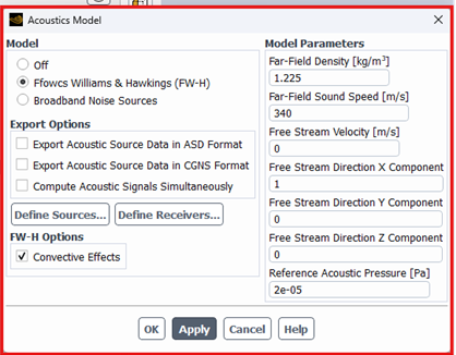
Figure 3: Locating the main acoustics panel in ANSYS Fluent via Problem Setup → Models → Acoustics → Edit.

In the Acoustics panel, select Ffowcs Williams & Hawkings. Let’s look at the critical options:

• Export Options: You can choose to Export Acoustic Source Data in ASD Format. This saves the pressure fluctuation data from your noise-generating surfaces. Consequently, you can use these .asd files for post-processing later without re-running the transient solver.
• Compute Acoustic Signals Simultaneously: This calculates the sound at your defined receivers while the CFD solver is running.

Next, you should define the noise sources and receivers. The Define Sources button opens a panel where you select the surfaces that generate noise (e.g., the blades of a wind turbine). The Define Receivers button lets you set up virtual microphones by entering their X, Y, and Z coordinates.

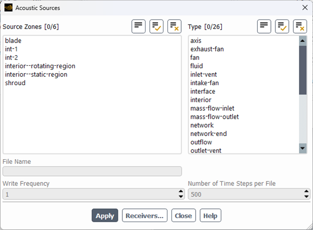
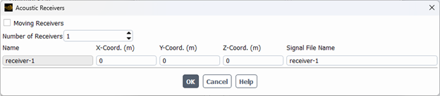
Figure 4: The Define Sources & Receivers panel. Here, users select noise-generating surfaces and set the coordinates of virtual microphones.

The final step is to configure the Model Parameters. These values are essential for the accuracy of the acoustic calculation.

• The Far-Field Density and Far-Field Sound Speed must match the properties of the fluid in the far field, which for most Aeroacoustics CFD problems is air (typically 1.225 kg/m³ and 340 m/s).
• For any simulation with a mean flow, you must enable Convective Effects to improve accuracy. This adds options to define the Free Stream Velocity and Direction.
• One of the most critical settings is the Reference Acoustic Pressure. The decibel (dB) scale is relative, so this value is vital. For noise in air, this must be set to 2e-05 Pascals. Using the default Fluent value will lead to incorrect Sound Pressure Level (SPL) results.
• Finally, the Source Correlation Length is a parameter used only for 2D simulations. It is an estimated length over which the 2D noise sources are correlated in the third dimension. The final SPL result is highly dependent on this estimated value, which makes it a source of uncertainty in 2D aeroacoustic analysis. This parameter is not required for 3D simulations.

For a practical example of this setup, explore our dedicated building aeroacoustics product case study. This tutorial shows the complete workflow, from setting up the transient simulation in ANSYS Fluent to post-processing the sound pressure level results.

Figure 5: Applying the FWH model to analyze sound pressure levels on a building facade.

Broadband Noise Sources Models

While the FWH model is excellent for detailed analysis of sound at specific locations, it requires a time-consuming transient calculation. For many engineering tasks, you first need to quickly identify where the noise is coming from. This is where the Broadband Noise Source models in ANSYS Fluent provide a huge advantage. These models are designed for fast acoustic analysis and are perfect for the early stages of design when you need to compare different concepts quickly.

The single most important highlight of this approach is its efficiency. Unlike the FWH model, the Broadband Noise models work with a steady-state flow solution. This means you can get valuable acoustic insights from a much faster RANS simulation, such as one using the k-epsilon or k-omega SST turbulence model. You simply run your steady-state simulation to convergence and then enable the acoustic model to post-process the results.

However, it is critical to understand the main limitation. As our reference explain, this method identifies the location and strength of noise sources, but it cannot predict the sound pressure signal at a distant receiver. Its purpose is to show you which parts of your geometry are the loudest, which you can see directly with contour plots of Acoustic Power Level (dB).

How to Set Up the Broadband Model

The setup for the broadband approach is very simple. After your steady-state flow solution has converged, navigate to the acoustics panel.

Figure 6: The main setup panel for the Broadband Noise Sources model in ANSYS Fluent. It features a simple interface that works perfectly with steady-state RANS solutions.

Select Broadband Noise Sources. You will notice a key difference from the FWH panel: there are no buttons to define sources or receivers. The software automatically uses the entire flow field as a potential source region.

The setup involves just a few key parameters:

• Reference Acoustic Power [W]: The broadband model calculates acoustic power (in Watts), not pressure. For accurate decibel calculations, this value must be set to 1e-12 Watts. This is the standard threshold of human hearing.
• Number of Realizations & Fourier Modes: These control statistical accuracy. Higher values give better results but take more time to post-process. The default values are a great starting point.

Getting Results: The true power of this model is visualization. In the Contours panel, you can plot variables like Acoustic Power Level (dB) on any surface. This will clearly show you the “hotspots” of noise generation.

Figure 7: A contour plot of Acoustic Power Level (dB) on a fan. This clearly identifies the blade tips as the primary noise hotspots.

 

Wave Equation Model

Sometimes, you need to see how sound behaves across your entire computational domain, not just at specific points. The Wave Equation model solves the acoustic wave equation directly on your CFD mesh. This gives you a full-field view of the sound pressure.

However, this method has strict rules:

• It requires a transient calculation.
• You must use the Second Order Implicit or Bounded Second Order Implicit time formulation.
• It is designed only for low Mach number flows where convective effects are negligible.

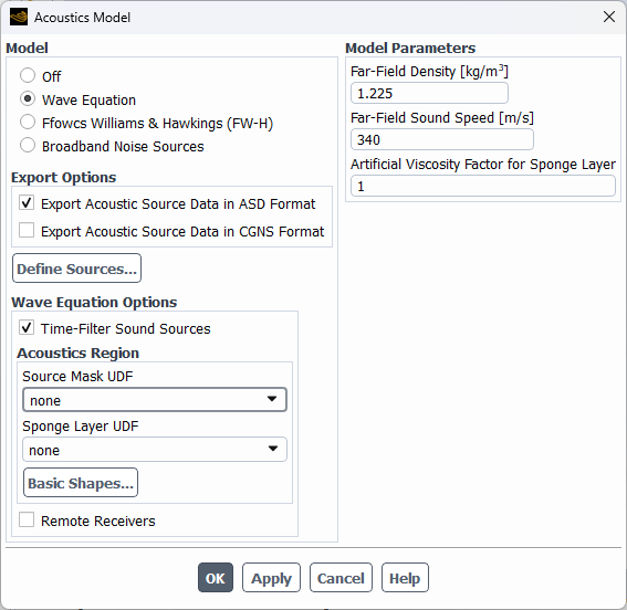
Figure 8: The setup panel for the Wave Equation model. Notice the Artificial Viscosity Factor, which prevents non-physical sound reflections from boundaries.

The panel contains several important parameters:

• Model Parameters: On the right, you set the basic fluid properties. Far-Field Density and Far-Field Sound Speed must match your fluid, which is typically air (1.225 kg/m³ and 340 m/s).
• Artificial Viscosity Factor for Sponge Layer: This is a key parameter for this model. By default, walls reflect acoustic waves. To prevent non-physical reflections from open boundaries, Fluent uses a “sponge layer” that absorbs sound waves. This parameter controls the strength of that absorption. The default value is 1. Increasing this value makes the layer absorb more sound, effectively making the boundary less reflective.
• Define Sources…: Similar to the FWH model, you can click this to select specific surfaces (like cylinder-wall) that act as the source of the noise.
• Acoustics Region: This section provides more advanced ways to define sources and absorbent regions. The Basic Shapes… button is a unique feature that allows you to define simple geometric regions (like a sphere or box) and designate them as either a sound source or a sponge layer. This offers great flexibility beyond just selecting existing boundaries.
• Wave Equation Options: The Time-Filter Sound Sources option applies a time-based filter to the acoustic sources. The transcript recommends leaving this disabled for typical industrial noise simulations to ensure all source effects are captured.

Setup and the FFT Trick:

In the setup panel, the Artificial Viscosity Factor for Sponge Layer is highly important. By default, walls reflect acoustic waves. Fluent uses a “sponge layer” to absorb sound waves at open boundaries. Increasing this value makes the layer absorb more sound.

A major limitation of the Wave Equation model is that it does not have a built-in tool for calculating SPL in decibels or performing an FFT analysis. However, there is a powerful post-processing trick:

1. After your Wave Equation calculation is complete, export the acoustic source data.
2. Go back to the Acoustics Model panel.
3. Change the model from Wave Equation to Ffowcs Williams & Hawkings (F-W-H). Do not re-run the calculation.
4. The Acoustic Signals button and the FFT tool are now available! You can load the source data files you just created and use the powerful FWH tools to get SPL plots and frequency spectrums.

Comparison: Which Acoustic Model Should You Use?

Each model has unique strengths. Choosing the correct model is the first step toward getting accurate results. The table below summarizes the key differences:

Feature	FWH Model	Broadband Noise Sources	Wave Equation
Primary Goal	Predicts SPL at specific far-field locations.	Identifies location and strength of noise hotspots.	Visualizes sound waves across the whole domain.
Required Flow	Transient (URANS, LES).	Steady-State (k-epsilon, k-omega).	Transient (Second-order implicit).
Receivers	Must define X, Y, Z coordinates.	No receivers. Points created via reports later.	The entire domain acts as a receiver.
Main Output	FFT Plots (SPL vs. Frequency).	Contour Plots (Acoustic Power Level dB).	Contour Plots (Sound Pressure).
Key Strength	Most accurate for far-away points.	Very fast diagnostic tool for design comparison.	Complete full-field visualization.
Limitation	Computationally expensive.	Cannot predict SPL at a distant point.	Low Mach numbers only; stationary mesh required.

 

Conclusion

Controlling noise is a critical part of modern engineering, and ANSYS Fluent provides a powerful suite of acoustic tools. The best model depends entirely on your goal:

• The FWH model is the standard for accuracy. Use it when you need precise SPL data in decibels at specific far-field locations.
• The Broadband Noise Sources model is the perfect diagnostic tool for speed. By working with a simple steady-state solution, it allows you to quickly identify the loudest hot spots on a body.
• The Wave Equation model provides a complete picture, calculating the sound field everywhere in your domain.

If you are struggling to set up these advanced physics models and need expert help, our engineering team is ready. We offer premium aeroacoustics CFD simulation tutorials to ensure your industrial projects are solved accurately and efficiently. Order your project today at CFDLAND.