

Noise is everywhere in the engineering world. In modern engineering, we use Computational Fluid Dynamics (CFD) not just to see how fluids flow, but also to analyze how they sound. To begin our blog into CFD acoustics, we must answer a fundamental question: what is aeroacoustics?
First, we must define basic acoustics. At its core, acoustics is the branch of physics that studies mechanical waves in gases, liquids, and solids. In simple terms, it is the science of sound. It deals with how sound is created, how it moves, and how it is received. Consequently, we can define the aeroacoustics meaning. Aeroacoustics is a specific branch of acoustics that focuses strictly on noise generated by the movement of a fluid. When a fluid, like air or water, moves in a turbulent way, it creates changes in pressure.
- Turbulent fluid flow is chaotic and unsteady.
- This chaotic motion creates pressure fluctuations.
- These pressure fluctuations travel away from the source as sound waves.
Therefore, an aeroacoustic simulation is the science of predicting sound that comes from fluid flow. The same fundamental equations of fluid dynamics that we use to calculate flow fields also contain the information needed to analyze the sound that the flow produces.

Figure 1: A visual diagram showing a turbulent flow from a jet engine exhaust with sound waves radiating outwards
The Physics of Sound: Basic Theory
To perform a meaningful aeroacoustic analysis, we need to understand the basic physics of sound. Sound is a physical phenomenon with properties we can measure and calculate.
More specifically, a sound wave is a series of rapid pressure fluctuations. Imagine dropping a stone in a calm pond; the ripples that travel outwards are like sound waves. In the air, these “ripples” are tiny, quick changes in the local pressure. In a CFD analysis, our main goal is to calculate these pressure fluctuations as they change over time and space.
Sound Intensity vs. Sound Pressure
When we talk about how “loud” a sound is, we are discussing its energy.
- Sound Intensity (I): The amount of energy the sound wave carries per unit of area (Watts/m²).
- Sound Pressure (p): The local pressure change caused by the sound wave. This is the SI unit of sound (measured in Pascals) that we calculate in CFD.
The most important relationship in aeroacoustics connects intensity directly to pressure:
\text{I} = \frac{p^2}{\rho c}
(Where I is Intensity, p is acoustic pressure, ρ is fluid density, and c is the speed of sound).

Figure 2: A schematic showing the definition of Sound Intensity. It represents the acoustic energy (power) flowing through a specific unit of area, a key metric for understanding the strength of a sound wave.
The Decibel (dB) Scale and SPL
The range of sound intensity that humans can hear is enormous. To solve this, we use the decibel (dB) scale, which makes large numbers easier to manage.
Because it is much easier to measure pressure than intensity, the standard way to describe noise is using the sound pressure level formula. Also measured in decibels (dB), the mathematical formula is:
\text{SPL} (\text{dB}) = 20 \log_{10} \left( \frac{p}{p_{\text{ref}}} \right)
Where I₀ is the reference sound intensity, which is set at the threshold of human hearing (the quietest possible sound we can hear).
Because it is much easier to measure pressure than intensity, the most common way to describe a noise level is using Sound Pressure Level (SPL). It is also measured in decibels (dB). The formula for SPL is very similar, but it uses pressure instead of intensity:
\text{SPL} (\text{dB}) = 20 \log_{10} \left( \frac{p}{p_{\text{ref}}} \right)

Figure 3: A chart comparing common sounds on the decibel (dB) scale. The logarithmic scale makes it easier to represent the huge range of sound levels we experience, from a quiet whisper to a loud jet engine.

Figure 4: A visualization of Sound Pressure Level (SPL). This is the standard measurement for noise in CFD and is calculated from the pressure fluctuations solved in the simulation.
Crucial Point: The Reference Pressure The value of the reference pressure (pref) changes depending on the fluid you are simulating. Setting this correctly in your CFD solver is essential for accurate dB results:
- For Air: pref = 20 micropascals (20×10−6 Pa)
- For Water: pref = 1 micropascal (1×10⁻⁶ Pa)
Aeroacoustics Fundamentals: How Flow Becomes Sound
A smooth, laminar flow is quiet. However, when a flow becomes turbulent, it is full of chaotic, swirling structures called eddies. These rapid pressure fluctuations created by turbulence are the direct source of sound waves.
The direct simulation of noise generation is extremely complex. However, as the founder of modern aeroacoustics equation 1950s, physicist Sir James Lighthill developed a revolutionary approach called the Lighthill acoustic analogy.

Figure 5: A portrait of Sir James Lighthill, whose pioneering work on the “acoustic analogy” provided the mathematical foundation
Instead of solving the full equations directly for sound, he rearranged them into a classic wave equation. The governing equation for the Lighthill acoustic analogy is:
\frac{\partial^2 \rho’}{\partial t^2} - c_0^2 \nabla^2 \rho’ = \frac{\partial^2 T_{ij}}{\partial x_i \partial x_j}
- Left Side (Wave Equation): Describes how sound waves propagate through a fluid.
- Right Side (Source Term): Contains the Lighthill stress tensor, which represents the fluid flow generating the noise.
Lighthill’s work helps us group sound sources into three main types:
- Monopole (Thickness Noise): Caused by a change in mass or volume (e.g., the exhaust of a jet engine).
- Dipole (Loading Noise): Caused by unsteady forces acting on a surface (e.g., a rotating propeller blade).
- Quadrupole (Shear Noise): Caused by the turbulent motion and shear within the fluid itself (e.g., mixing noise in a high-speed jet stream).
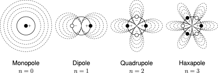
Figure 6: An illustration of the three primary aeroacoustic sound sources. The pulsating sphere (monopole), the surface with unsteady forces (dipole), and the turbulent eddy (quadrupole) are the building blocks of noise generation in fluid flow.
Overview of Computational Acoustic Modeling Approaches
When engineers perform an acoustic simulation, there is not just one way to solve the equations. The choice depends on the required accuracy, computational power, and the location of the noise. Computational methods are generally divided into three main families:
- The Direct Method (DAS): This approach solves the fluid flow and the sound generation simultaneously. It is highly accurate but requires massive computational power (like DNS or LES). It is best for near-field acoustics.
- The Hybrid Methods: This is the most common industrial approach. First, the software solves the fluid flow using a standard transient CFD simulation. Then, it uses that flow data to calculate the sound propagation separately. Popular hybrid models include the Ffowcs Williams-Hawkings (FW-H) integral method for open spaces, and the Wave Equation for enclosed spaces (like ducts).
- Broadband Noise Source Models: These models use a fast, steady-state flow solution to estimate the overall sound power and quickly locate noise “hotspots” without running expensive transient calculations.
To learn how to select and apply these specific methodologies inside industrial software, read our complete Acoustic Models in ANSYS Fluent.
From Time to Frequency: The Importance of FFT
When we run a transient simulation, our direct result is a pressure signal showing how pressure changes over time. However, looking at a wavy line in the time domain does not tell us much about the character of the noise. To truly understand the sound, we must analyze the frequency vs time domain. We need to know which frequencies are present and which are the loudest. This allows us to answer critical engineering questions:
- What are the dominant frequencies in the noise?
- Is the noise a low-frequency rumble or a high-frequency whistle?
- Is it a sharp tone (tonal noise) or spread out (broadband noise)?
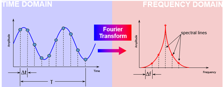
Figure 7: A complex pressure signal over time (left) is transformed into a simple frequency plot (right), revealing the dominant noise frequencies that are otherwise hidden
The mathematical process for converting a signal from the time domain to the frequency domain is called a Fourier Transform. Because doing this by hand is difficult, CFD software uses a fast algorithm to perform an FFT analysis (Fast Fourier Transform). The FFT analysis takes the raw pressure data and creates a clear Sound Pressure Level (SPL) frequency spectrum. The peaks on this new plot immediately show engineers the exact problem frequencies they need to fix.


Figure 8: A sample Sound Pressure Level (SPL) plot from an ANSYS Fluent acoustic analysis. The peaks on the graph clearly show the dominant frequencies in the noise, helping engineers pinpoint the source of the problem.
Where Aeroacoustics CFD is Used (Applications)
These fundamental physics and simulation techniques are used every day to solve real-world industrial noise problems. Below are the most common applications of acoustic CFD:
- Wind Turbine Noise: The spinning blades of wind turbines create complex airflow patterns that produce significant noise, especially near residential zones. Engineers use advanced Two-Way Fluid-Structure Interaction (FSI) coupled with acoustic models to ensure structural safety while minimizing noise. Learn more in our wind turbine noise CFD simulation tutorial.
- Silencers and Mufflers: Noise from fans in ventilation systems is a common problem in buildings. By analyzing transmission loss (TL) and sound pressure contours, engineers can optimize internal geometries and sound-absorbing materials. Explore this process in our muffler CFD simulation guide.
- Propeller Noise: Traditional drone and marine propellers can be highly disruptive. By utilizing advanced geometries, such as toroidal shapes, engineers can dramatically reduce dipole loading noise while maintaining thrust. See this applied in our propeller aeroacoustics CFD project.
- Building Aeroacoustics: When strong wind flows around tall buildings, it creates annoying whistling or roaring sounds for residents. Simulating the wind flow allows architects to identify noisy facade elements and round sharp corners before construction begins. Read about building aeroacoustics here.
- Turbomachinery and Fans: Fast-spinning blades in industrial pumps and cooling fans create a harsh mix of tonal humming and broadband “whoosh” sounds. CFD allows engineers to target specific problem frequencies and alter blade counts to quiet the machine. Learn how in our fan noise CFD simulation breakdown.
- Supersonic Jet Noise: The turbulent mixing and shock waves from a supersonic aircraft create some of the loudest sounds in engineering. Detailed Large Eddy Simulations (LES) allow designers to visualize acoustic pressure fluctuations and redesign exhaust nozzles. Discover the details in our supersonic jet noise CFD analysis.
Another perfect example of this is the design of modern propellers. Traditional propellers can be very noisy. Using Aeroacoustics analysis, engineers can simulate new designs, like the toroidal propeller, to significantly reduce the generated noise while maintaining performance. You can explore a detailed simulation of this advanced application in our Toroidal Propeller Aeroacoustics Simulation using Broadband Noise Sources Model tutorial.


Figure 9: By predicting noise with CFD, we can solve noise problems at the design stage, saving time and money


Figure 10: Some aeroacoustics examples from our library
Conclusion
In this guide, we have covered the essential foundations of fluid-driven noise. We started with the basic physics of sound pressure, explored how turbulent flow generates noise through Lighthill’s analogy, and reviewed the primary computational methods used in modern engineering. Finally, we saw how FFT analysis turns complex time-domain signals into actionable frequency data.
If you are dealing with complex noise generation in your industrial designs and need professional assistance, CFDLAND can help. Explore our aeroacoustics CFD simulation services to see how we can predict, analyze, and solve your noise problems before manufacturing begins.