
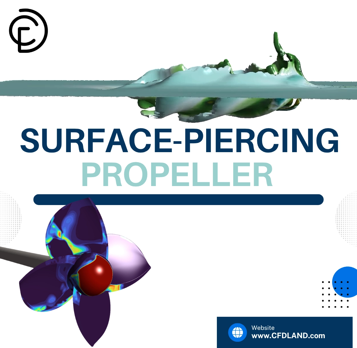
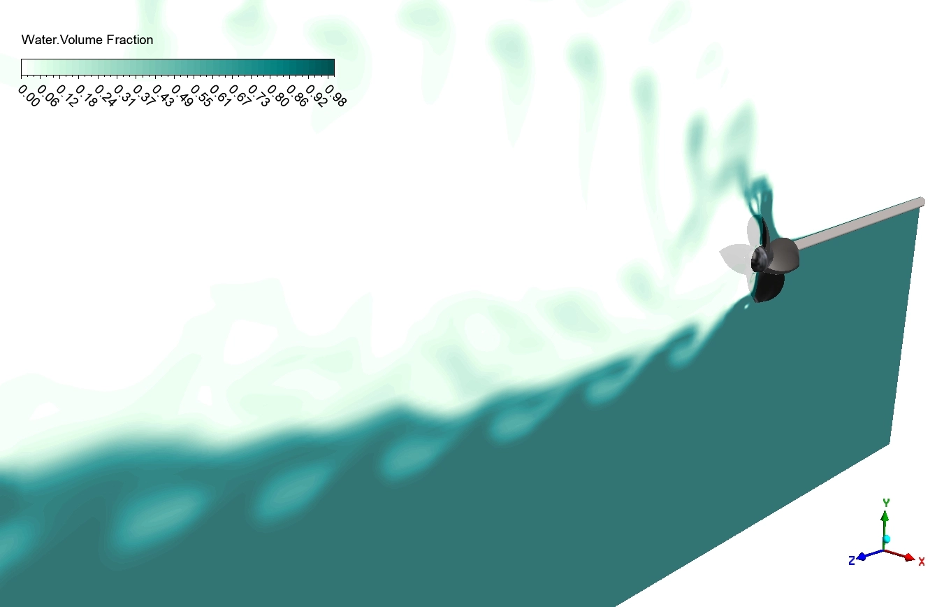
A surface-piercing propeller operates half in the air and half in the water. This split environment makes the fluid flow very difficult to predict. The spinning blades smash into the heavy water and drag thin air down with them. This creates severe splashing and large air pockets.
To design better boat parts safely, we use a CFD simulation project to test these forces. We base our computational domain directly on the respected academic paper by Kamran et al. By following their physical setup, this ANSYS Fluent tutorial teaches you how to accurately calculate the pushing force, the spinning resistance, and the overall propeller efficiency.
- Reference [1]: Kamran, M., N. M. Nouri, and H. Askarpour. “Numerical Investigation of the Effect of Trailing Edge Shape on Surface-Piercing Propeller Performance.” Applied Ocean Research125 (2022): 103230.
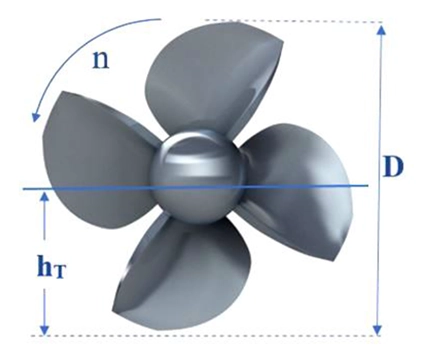
Figure 1: The physical geometry of the surface-piercing propeller. [1]
Simulation Process: VOF Setup in Propeller CFD Simulation
We constructed a large rectangular tank around the propeller to capture the air-water mixture. The domain was discretized using a fine mesh comprising 7,468,230 cells, enabling ANSYS Fluent to accurately resolve the sharp interface between the two phases. A combination of hexahedral elements was used outside the rotating region, while polyhedral elements were employed within the rotating region.
The blades rotate at a constant speed of 251 rpm. To make the solid parts spin correctly, we use the sliding mesh technique. Because the tank contains both air and water, we apply the transient Volume of Fluid (VOF) model. This specific mathematical method tracks the free surface boundary as the blades cut through it. You can find more similar rotating equipment simulation in our Turbomachinery tutorials section. In fact, our final objective here is to extract torque, Kt, Kq, and efficiency values from the Fluent solution to evaluate overall propeller performance.
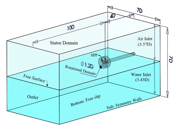
Figure 2: The computational domain featuring the air inlet, water inlet, and free surface boundary
Post-processing: Evaluation of Hydrodynamic Forces and Propeller Efficiency
The primary goal of this simulation is to extract the hydrodynamic forces. To evaluate the propeller performance, we calculate the hydrodynamic forces and apply standard marine formulas. The spinning blades generate a raw thrust of 522.21 N and a torque resistance of 12.747 N.m. Using the advanced formulas below, we find a thrust coefficient of 0.156 and a torque coefficient of 0.0152.
J = \frac{V_a}{nD}
K_T = \frac{T}{\rho \cdot n^2 \cdot D^4}
K_Q = \frac{Q}{\rho \cdot n^2 \cdot D^5}
\eta = \frac{K_T}{K_Q} \cdot \frac{J}{2\pi}
Where J is advance ratio, T is thrust force (N), Q is torque (N·m), ρ is water density, n is rotational speed (rps), and D is propeller diameter (m).
| Parameter | Symbol | Value | Unit |
| Thrust | T | 522.21 | N |
| Torque | Q | 12.747 | N·m |
| Thrust Coefficient | KT | 0.156 | – |
| Torque Coefficient | KQ | 0.0152 | – |
| Efficiency | η | 16.08 | – |
Note that, we only continued the solution for a very limited time due to its high computation burden. Given the tutorial purposes, we can calculate torque and thrust coefficients with the given data, but there would be surely differences compared to paper data. You need to continue the solution for a longer time until the propeller reaches steady state condition.
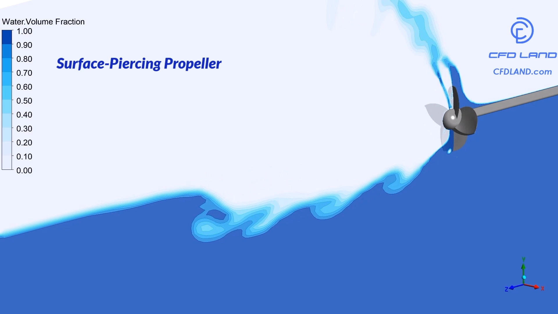
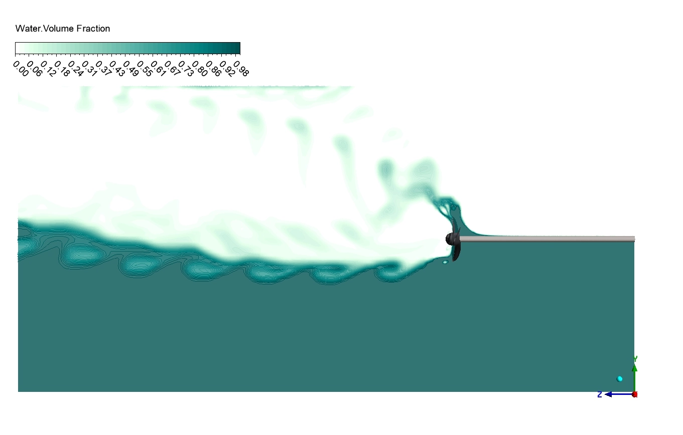
Beyond the numbers, we must analyze the contours to understand the fluid physics. First, we look at the water volume fraction contour. When the blades slice through the calm liquid, they push a heavy splash backward. This displacement creates a visible dry trough directly behind the propeller.
Figure 3 The water surface deformation showing the physical trough created by the spinning blades.
Alt Text: Water volume fraction contour showing a large splash and a dry gap behind the propeller.
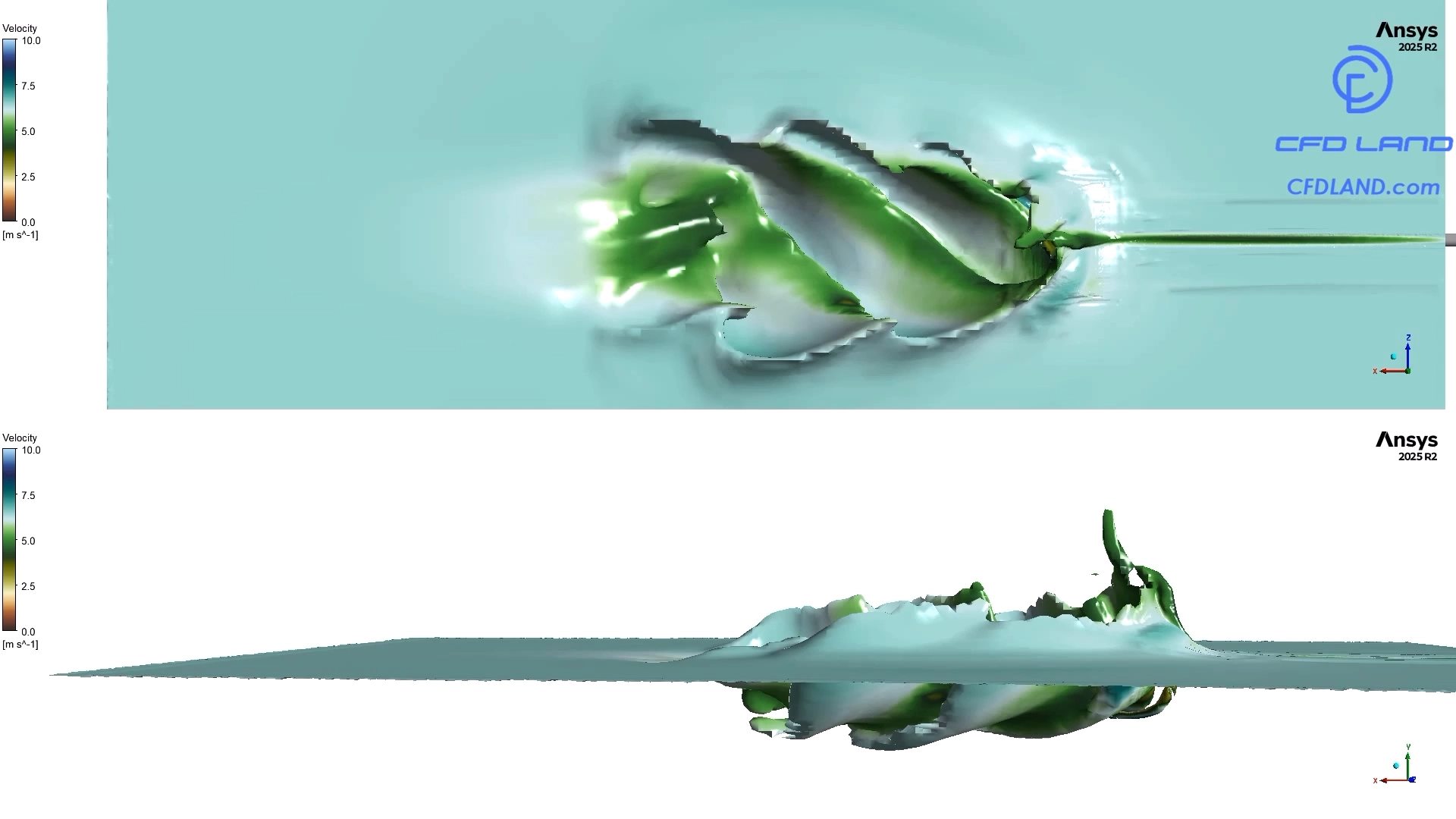
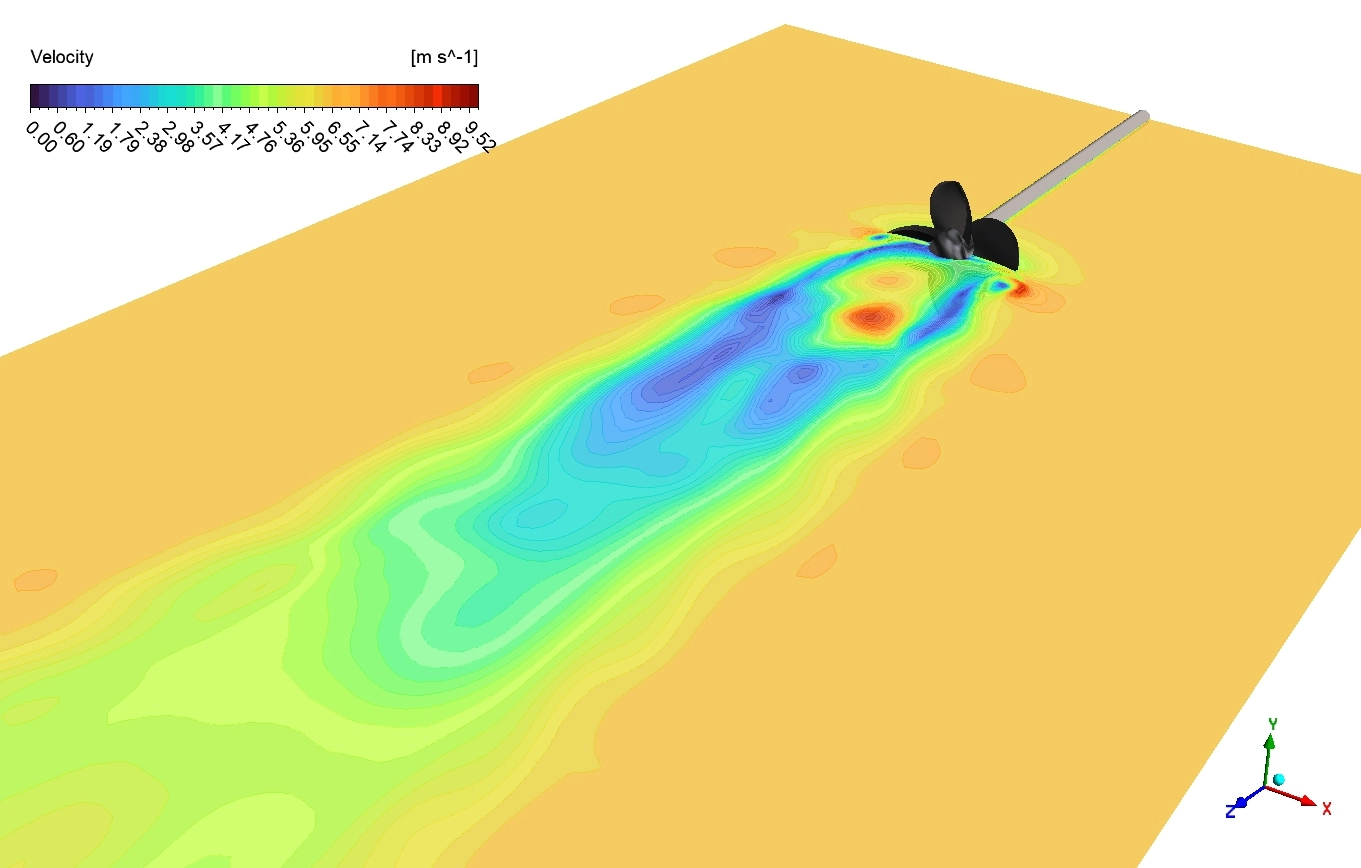
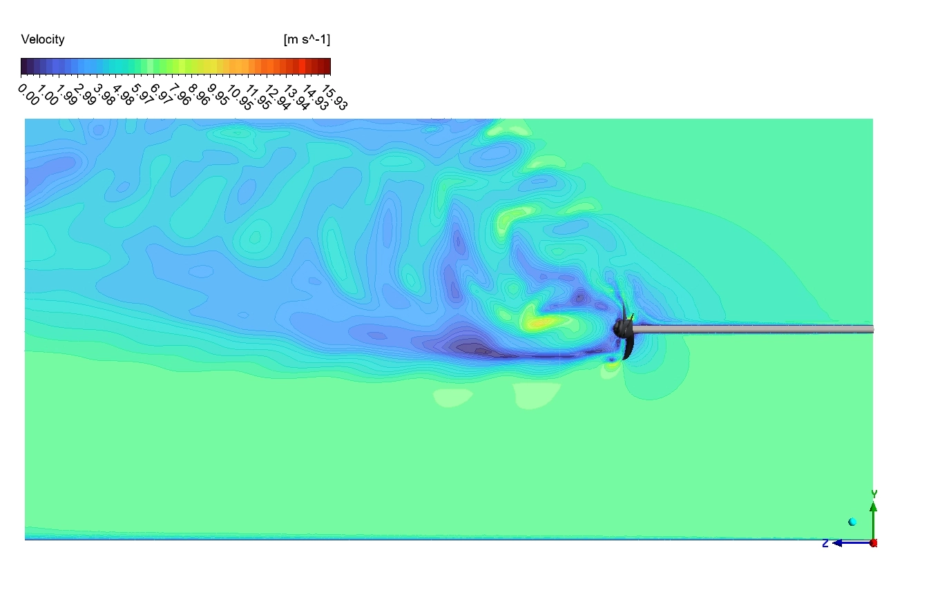
The velocity contour is plotted on an iso-surface representing the air–water interface. The figure illustrates the velocity distribution and the deformation of the free surface in the vicinity of and downstream of the propeller. The helical pattern observed behind the propeller reflects the interaction between the propeller-induced flow and the air–water interface. The maximum velocity on the displayed iso-surface reaches approximately 10.0 m/s, with the highest velocities occurring near the propeller and within its wake.
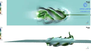
Figure 4: Velocity contour on an iso-surface representing the air–water interface, showing the free-surface deformation and propeller-induced wake.
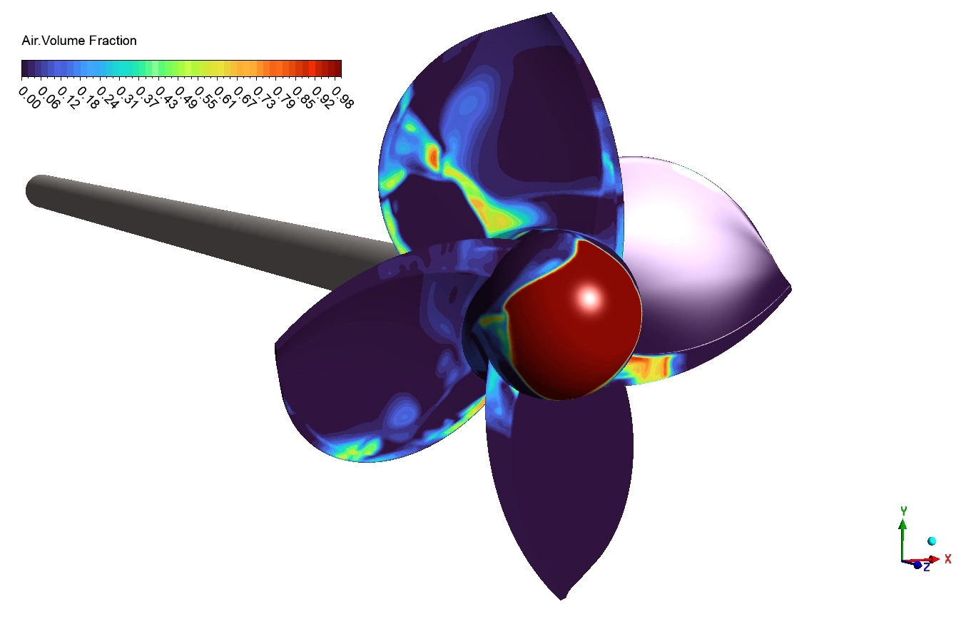
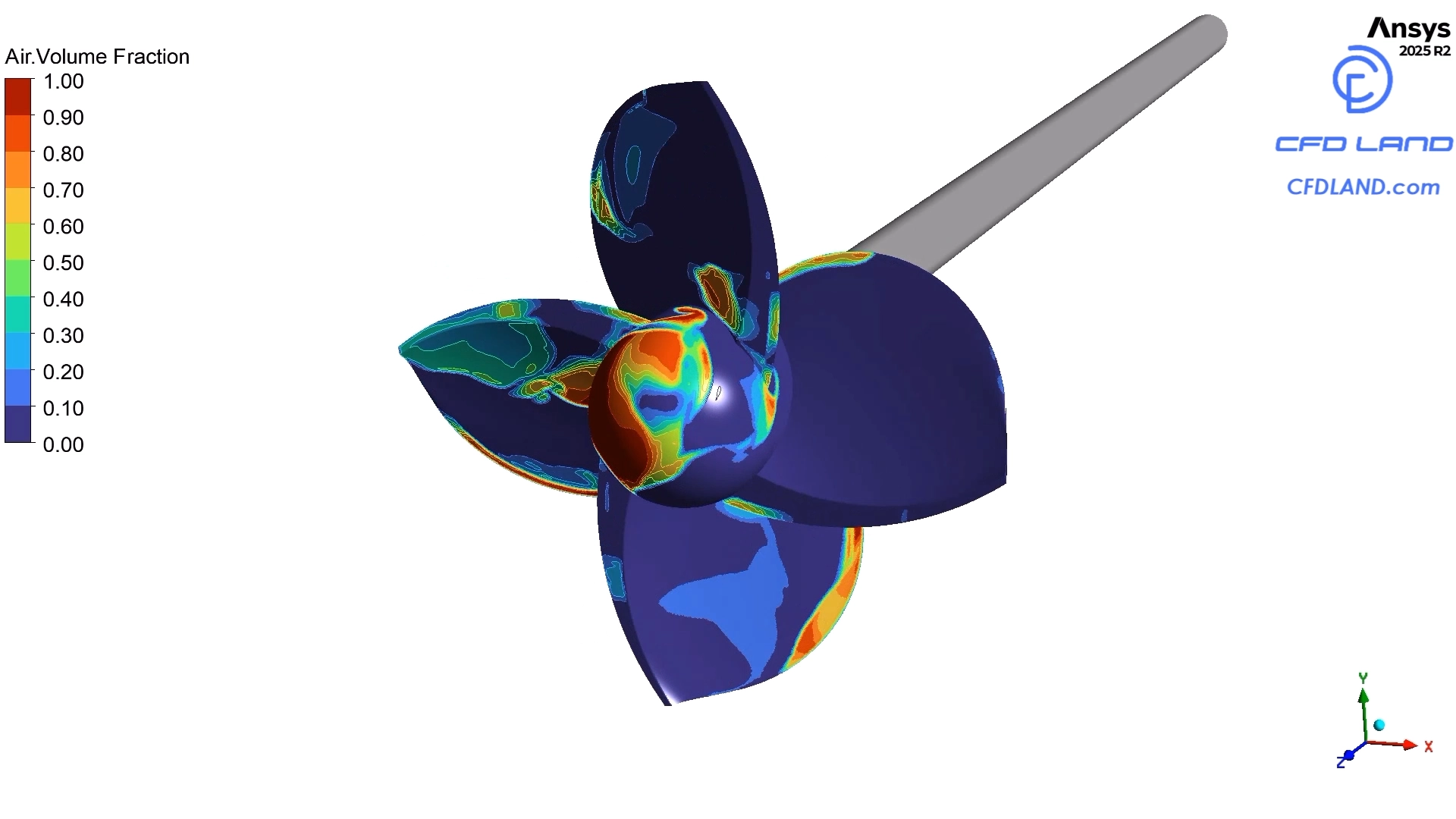
Lastly, we examine the air volume fraction strictly on the propeller surface. This contour explains the ventilation physics. The image shows deep red areas with a maximum fraction value of 1 near the hub and the blade root. This means pure air is being sucked heavily down the back of the blades. This trapped air pocket reduces the water friction but also changes the thrust load. This strong physical ventilation confirms our computational setup behaves like a real high-speed boat.
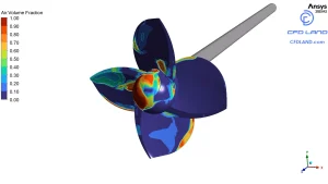
Figure 5: The ventilation physics showing pure air sucked deeply down the back of the blades.
FAQ About Propeller Performance Physics
- Why does the air volume fraction reach 1 near the propeller hub? When the blades break the water surface at high speed, they pull air down with them. The low pressure behind the thick blade root sucks this air inward, creating a pocket of pure air known as ventilation.
- What does the helical wake in the Q-criterion contour show? The blades slice the water and spin it backward. This pushing action creates swirling tubes of water called vortices. The helical shape proves the rotational energy from the engine is correctly transferring into the surrounding fluid.
- Why do we use a sliding mesh technique for this CFD project? A surface-piercing propeller constantly moves back and forth between dense water and light air. A sliding mesh physically rotates the computational grid in the simulation, capturing the true dynamic forces as the blades crash into the water surface during every single rotation.







Reviews
There are no reviews yet.