When an object flies faster than the speed of sound, it hits a solid wall of air. This creates a massive wave of high pressure called a bow shock. Predicting the exact distance between this shock wave and the object is a critical engineering problem. If aerospace engineers calculate this distance incorrectly, the extreme heat and drag will physically destroy the flying vehicle.

In this tutorial, we solve this exact problem using the ANSYS Fluent density-based solver. We will run a compressible Navier-Stokes simulation to capture the violent aerodynamics around a blunt sphere. If you want to master high-speed flows, studying our Fluid Mechanics CFD tutorials is your best next step. Today, you will see exactly how the shock stand-off distance changes as the freestream speed increases.

• Reference [1]: Nagata, T., et al. “Investigation on subsonic to supersonic flow around a sphere at low Reynolds number of between 50 and 300 by direct numerical simulation.” Physics of Fluids5 (2016).

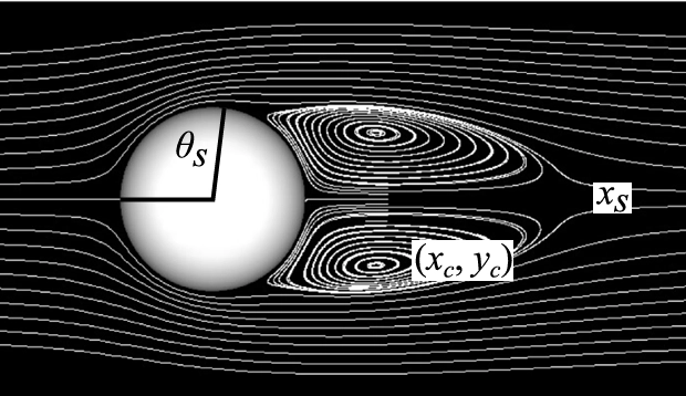
Figure 1: The physical geometry diagram defining the separation angle, separation length, and recirculation wake center. [1]

Simulation Process: Exact Validation Setup

To capture the exact bow shock, we require a highly controlled physical domain. We use ANSYS Meshing to build a 2D space. We generate a fully structured O-grid. This specific mesh topology aligns the cell faces perfectly with the expected shock wave direction. This minimizes numerical diffusion errors. We set up the density-based solver in ANSYS Fluent to handle the high-density gradients. We test the flow across multiple speeds. We increase the freestream Mach number from exactly 1.05 to 2.0. Our main validation goal is to track the shock stand-off distance (Lshock/D) and compare the ANSYS Fluent output directly against published DNS reference data.

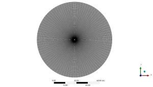
Figure 2: The structured O-grid topology created in ANSYS Meshing, featuring high cell density near the stagnation point.

Post-processing: Deep Physics of Bow Shocks and Wake Separation

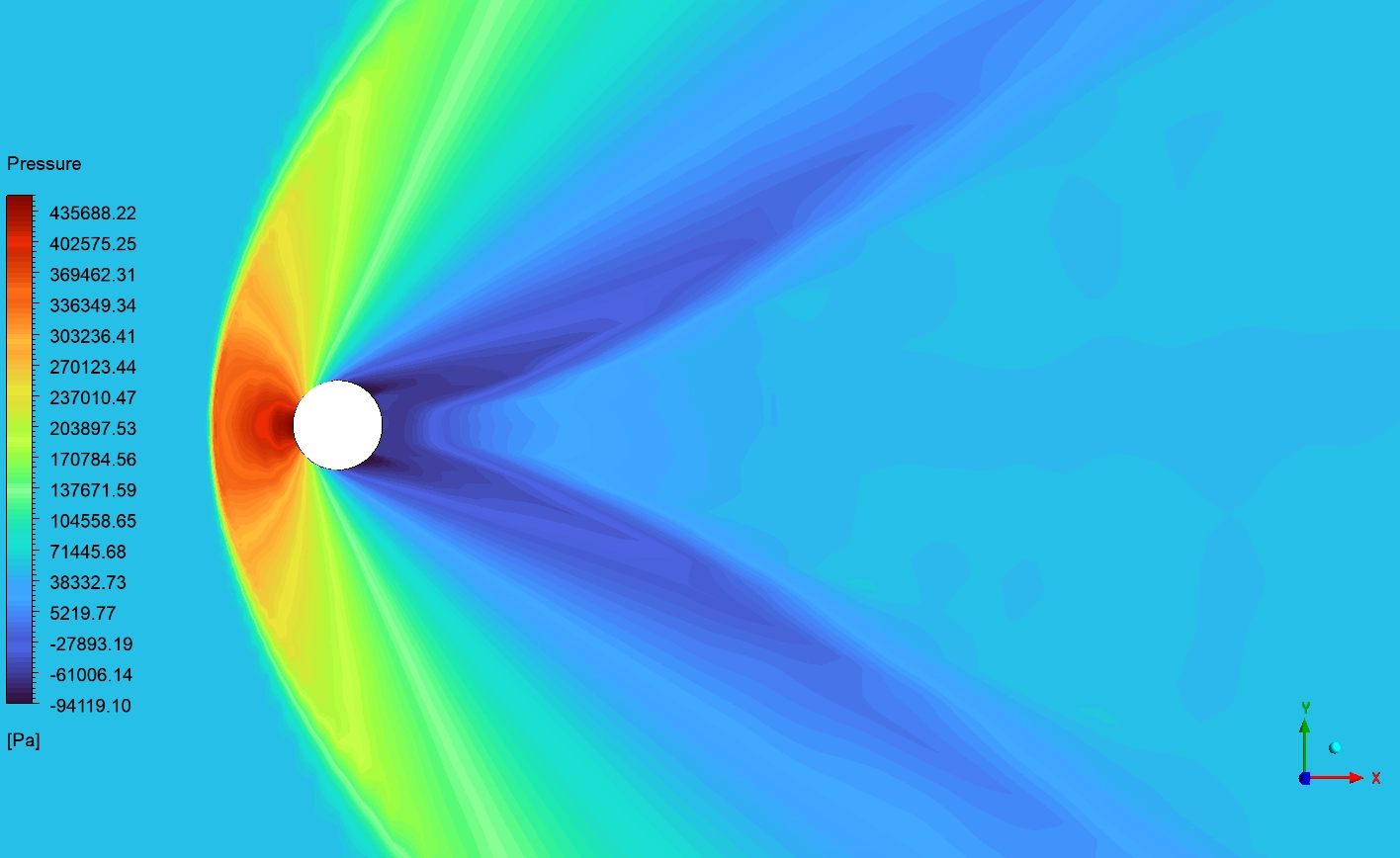
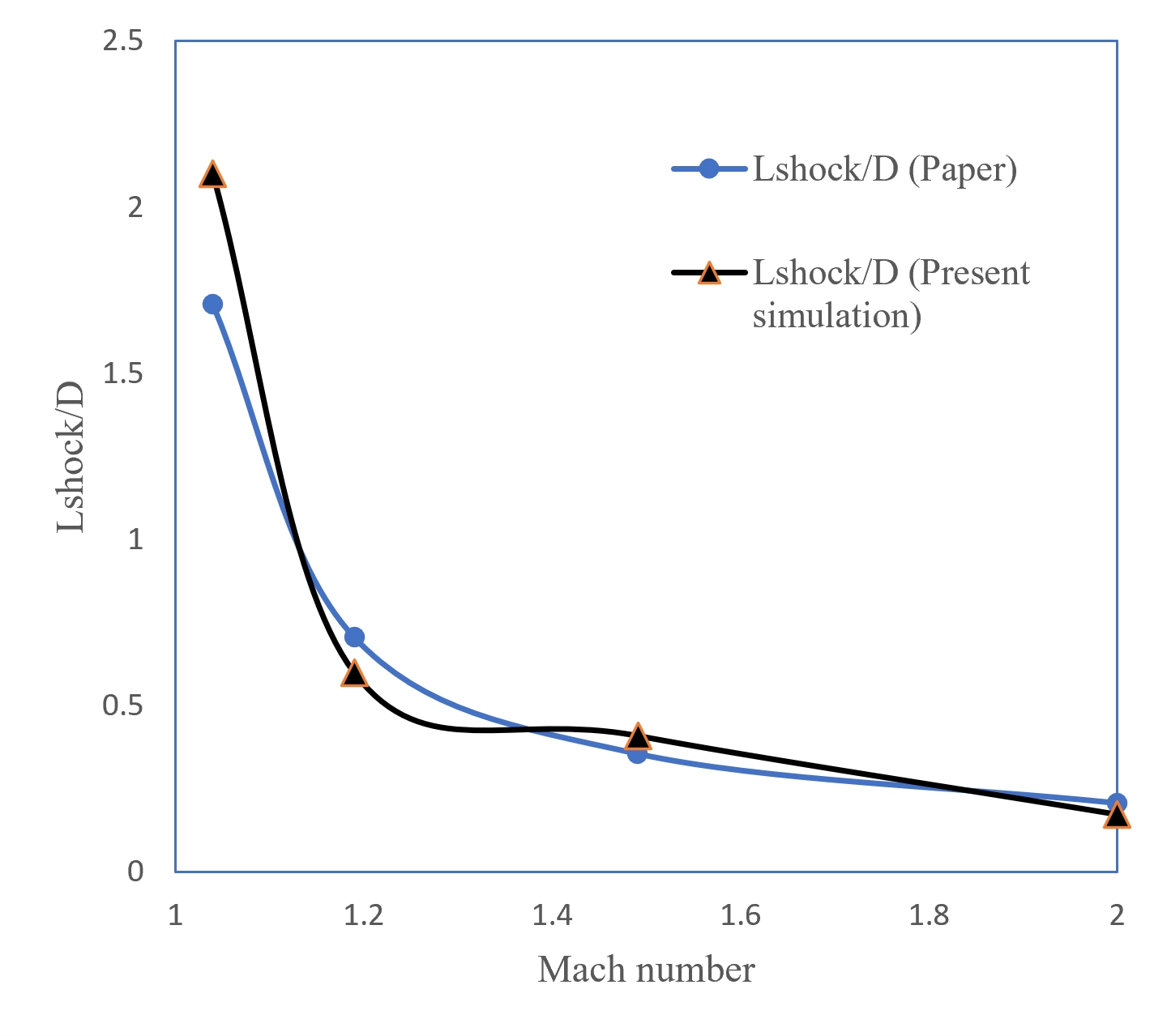
We must now study the visual contours and graphs extracted from ANSYS Fluent. We will analyze exactly how the supersonic air decelerates, compresses, and separates as it strikes the sphere. Look closely at the graph in Figure 3. The horizontal axis represents the Mach number increasing from exactly 1.05 to 2.0. The vertical axis tracks the Lshock/D ratio. The blue line is the exact DNS reference data. The black line is our ANSYS Fluent CFD output.

Notice the massive drop on the left side of the graph. At Mach 1.05, the flow is barely supersonic. The bow shock sits very far away from the sphere, creating a large Lshock/D value. As the Mach number accelerates toward 2.0, the black line drops sharply. The extreme speed forces the bow shock to move violently closer to the solid surface. Our ANSYS Fluent data matches the blue reference data perfectly at exactly Mach 1.2 and Mach 2.0.

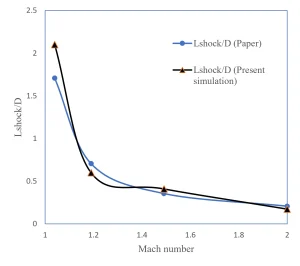
Figure 3: The validation plot proving the ANSYS Fluent solver perfectly captures the Lshock/D drop from Mach 1.05 to 2.0.

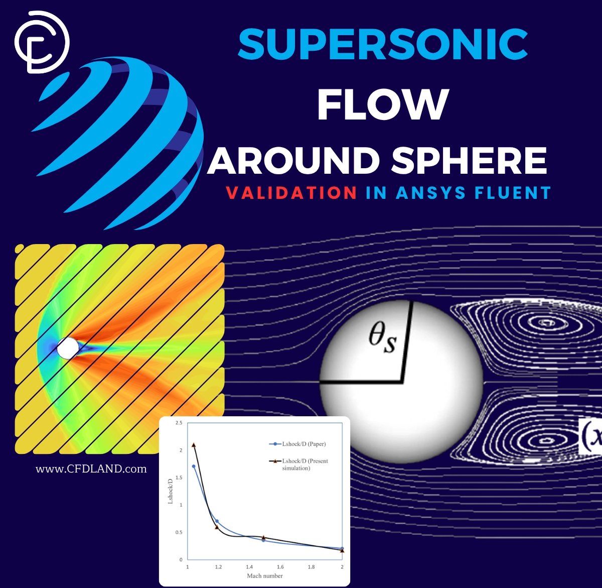
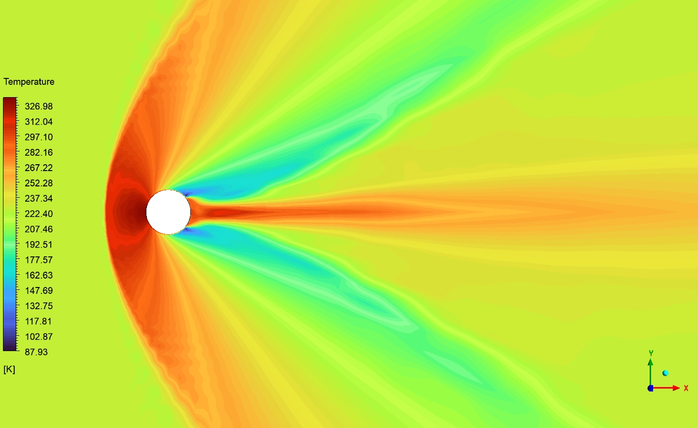
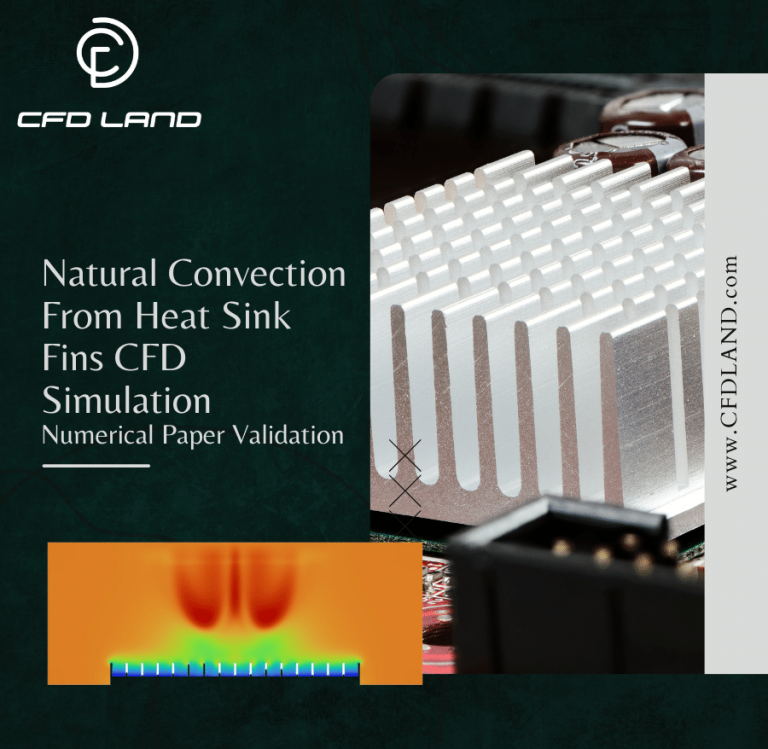
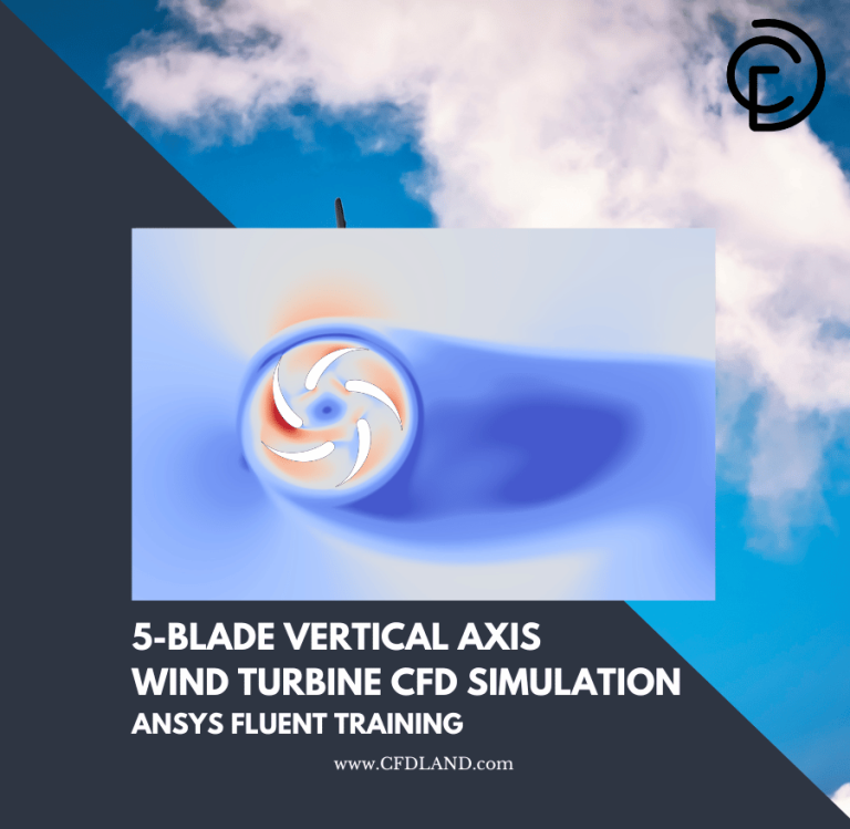
Now look at Figure 4. This is the Velocity magnitude contour. The color legend tracks the air speed from exactly 0.00 to 682.57 m/s. The supersonic air approaches from the left. Directly in front of the sphere, you see a thick green and blue curved wall. This is the detached bow shock. The absolute tip of the sphere is dark blue. Here, the air speed drops instantly to zero. This is called the stagnation point. Because the air cannot go through the solid metal, it comes to a complete, violent stop. The kinetic energy of the speed converts instantly into extreme static pressure. After hitting the wall, the air escapes around the top and bottom edges, turning bright red as it accelerates rapidly to 682.57 m/s.

Figure 4:  The Velocity magnitude contour proving the upstream air decelerates from 682.57 [m s^-1] to 0.00 [m s^-1].

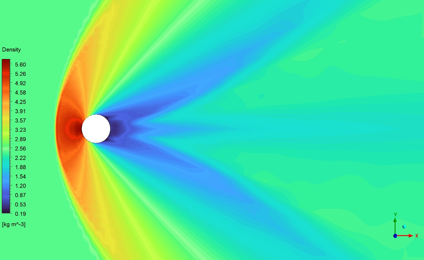
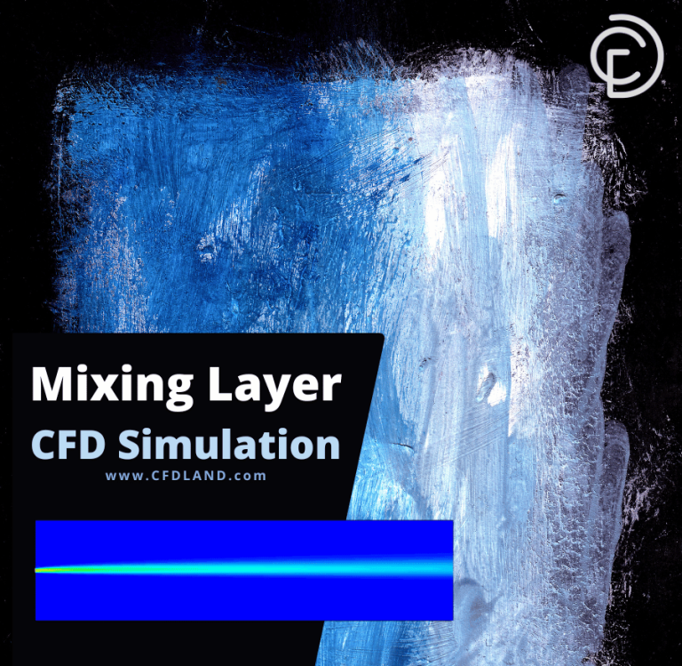
Finally, this graph proves exactly how much physical force hits the object. The horizontal axis maps the physical surface position from exactly -0.5 to 0.5 [m]. The vertical axis maps the Static Pressure from exactly -100,000 to 500,000 [Pa]. Look at the peak on the far left. At position x = -0.5 [m] (the exact front tip), the pressure explodes upward to nearly 450,000 [Pa]. This massive pressure spike is the direct physical result of the bow shock impact. As the air flows over the curved sides, the black line drops sharply below 0 [Pa]. Finally, notice the tiny bump between exactly x = 0.35 and 0.40 [m]. This small rise in pressure proves that ANSYS Fluent successfully captured the wake compression and reattachment shock at the rear of the sphere.

Figure 5: The wall Static Pressure graph proving the bow shock impact creates a massive peak force near 450,000 [Pa].

Frequently Asked Questions (FAQ)

•  Why is the bow shock stand-off distance important in supersonic flow simulations?
  • The bow shock stand-off distance determines how far the detached shock wave forms ahead of a blunt body. This parameter directly affects aerodynamic drag, pressure loading, and aerodynamic heating. Accurate prediction of the shock stand-off distance is essential for the design of high-speed aerospace vehicles, re-entry capsules, and supersonic projectiles.
• Why is the density-based solver used for this ANSYS Fluent simulation?
  • The density-based solver is specifically designed for compressible flows with strong pressure and density gradients. Since supersonic flow around a sphere generates a detached bow shock, the density-based approach provides better numerical stability and accuracy for capturing shock waves compared to pressure-based methods.
• How does the bow shock location change as the Mach number increases?
  • As the freestream Mach number increases, the detached bow shock moves closer to the sphere surface. Near Mach 1, the shock stands relatively far from the body, resulting in a larger shock stand-off distance. At higher Mach numbers, the stronger compression causes the shock wave to become more compact and approach the sphere, reducing the shock stand-off distance.