
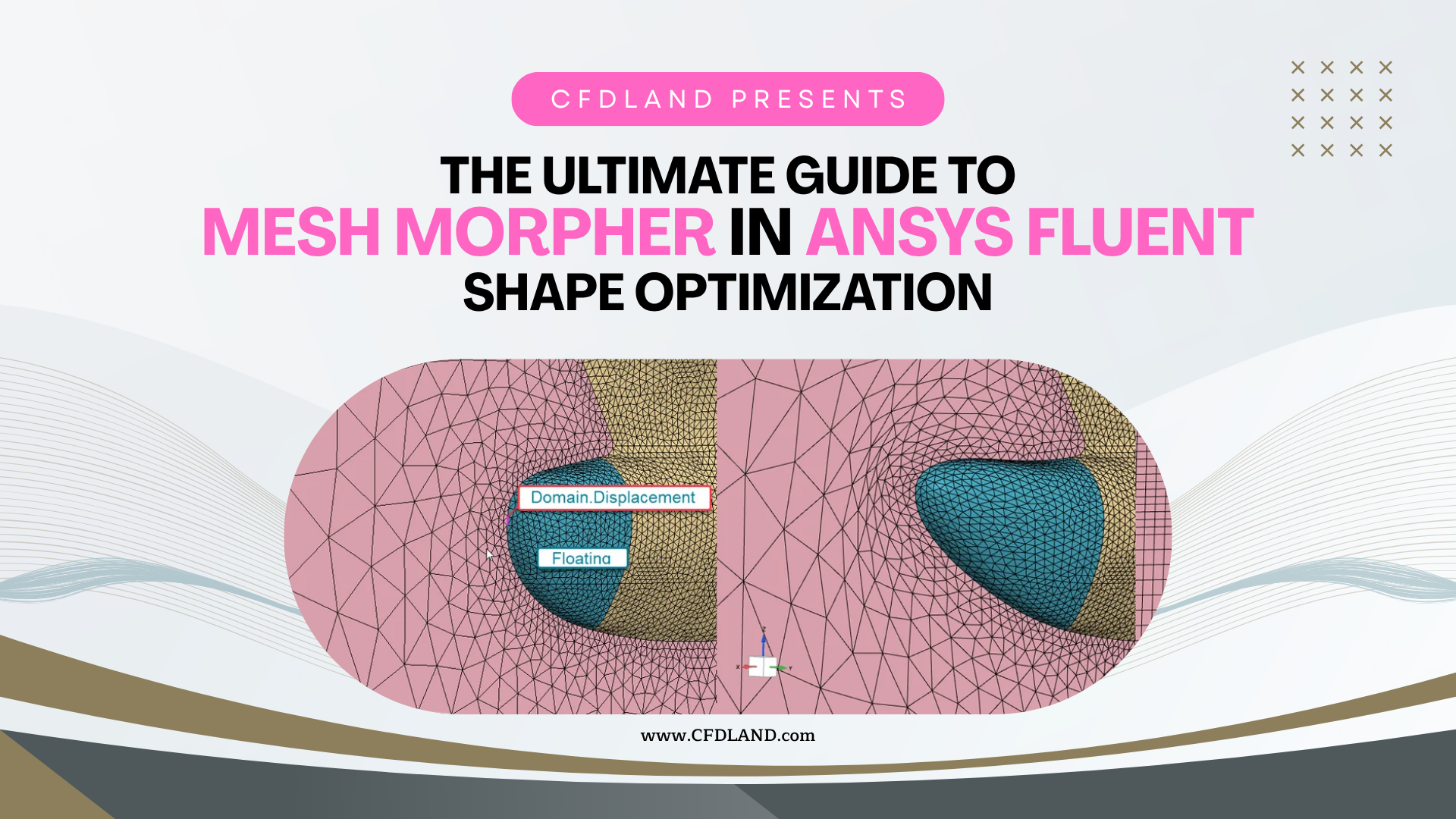
When you design a part, you usually want to find the best shape for it. Normally, if you want to test a new shape, you must draw it again and make a new mesh. This takes a lot of time. To fix this problem, ANSYS Fluent uses a tool called the Mesh Morpher/Optimizer. This tool automatically changes the shape of your old mesh to find a better design. It uses a simple method called direct search. It does not use complex math or hard derivatives. It only looks at the final result and tries to find a better shape step by step. We previously wrote a full guide about the complex math method. You can read it here: Adjoint Solver in ANSYS Fluent: The Ultimate Guide to Shape Optimization. But in this blog, we will only focus on the simple Mesh Morpher and its different models.
Figure 1: Adjoint Solver in ANSYS Fluent: The Ultimate Guide to Shape Optimization
We use an example to see how the methods work. We will use a 3D spiral duct system. You can see the main problem in our Duct System Optimization Tutorial. In this example, air goes into a square pipe, turns inside a spiral shape, and comes out. We want to find the best shape to make the air flow better and reduce the pressure drop. We will use the Mesh Morpher to stretch and move the mesh automatically. We will test the different optimizer models on this duct to see which method finds the best shape.
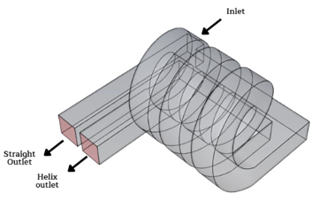
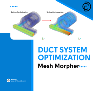
Figure 2: A guide example to investigate different optimizer models
Mesh Morpher vs Adjoint Solver: Which One & When?
ANSYS Fluent has two main tools to find the best shape for your design: the Adjoint Solver and the Mesh Morpher/Optimizer. They both try to improve your geometry, but they use very different math. You must know the difference so you can choose the right tool for your specific CFD project. The main difference is how they decide to change the shape. The Adjoint Solver uses complex math called gradients, while the Mesh Morpher uses a simpler method called direct search.
First, let us look at the Adjoint Solver. This tool calculates the exact math derivative for every single point on the wall. It tells the software exactly where to pull or push the shape to get a better result. This method is very fast when you have thousands of parameters. It is best to use this tool when you have a free-form shape and you do not know what the final design should look like. However, the math is very complex, and sometimes it can fail if the problem is not smooth.
On the other hand, the Mesh Morpher is much simpler and safer. It does not calculate complex derivatives. Instead, it changes the shape slightly using control points and then looks at the final result. If the new result is better, it keeps the shape. Because it does not use complex math, it is very robust and does not crash easily. It is the best choice when math derivatives are impossible to calculate. But, it has some important limits. For example, ANSYS clearly states that you cannot use the Mesh Morpher with a Dynamic Mesh or a sliding mesh.
To make it easy to choose, we made a quick guide table below. You can look at this table before you start your next optimization project.
Quick Guide: Adjoint Solver vs Mesh Morpher
| Feature | Adjoint Solver | Mesh Morpher / Optimizer |
| Math Method | Gradient-based (Uses complex derivatives) | Non-gradient (Uses simple direct search) |
| Best Used For | Free-form shapes, unknown final designs | Specific parameter changes, difficult math problems |
| Main Limitation | Hard to set up, needs smooth gradients | Cannot be used with Dynamic Mesh |
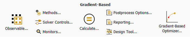
6 Optimizers and Our Duct Example Results
When you open the Optimizer tab in the Mesh Morpher window, you must choose a mathematical model to guide the shape changes. ANSYS Fluent provides six built-in direct search methods. Before running any of these methods, it is absolutely critical to check the box for Reject Poor Quality Meshes and set the Minimum Orthogonal Quality to 0.05. This safety step ensures that the moving mesh does not crash or break during the shape deformation process. To evaluate the performance of each optimization method, we applied them to our 3D duct case study. Below, we explain the simple theory behind each model and report the essential outputs for every method.
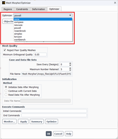
Figure 3: The Optimizer tab in ANSYS Fluent. Always set the Minimum Orthogonal Quality to 0.05 to protect your mesh
NEWUOA model
First, let us look at the NEWUOA model. We did not test this model in our duct example because it requires a special User-Defined Function (UDF) to work properly. However, you should know that it is a very fast and accurate model. It builds a mathematical approximation inside a safe zone called a trust region. ANSYS strongly recommends this model for projects that have a large number of parameters.
Compass optimizer
Next, we tested the Compass optimizer. This model changes the parameters one by one in positive and negative directions. If it finds a bad result, it cuts the step size in half and tries again. In our duct test, the Compass method finished after 33 runs. It successfully reached a final objective function of 0.94238611. The graph shows some large changes at the beginning, but it slowly becomes flat and completely stable at the end.
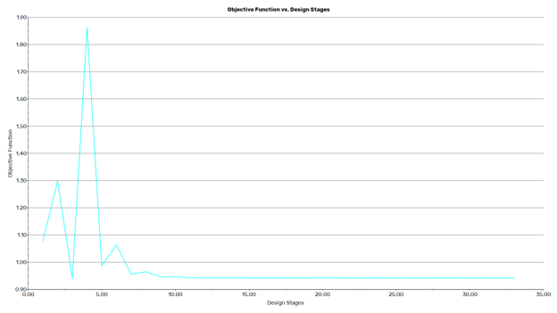
Figure 4: The Compass optimizer took 33 runs to find the final shape, reaching an objective function of 0.94238611
Powell optimizer
After that, we used the Powell optimizer. This model searches for the best shape by moving in straight, perpendicular lines. This smart movement stops the model from ruining a good result it already found in a previous step. For this test, we set the Max Number of Designs to 500 and the Tolerance to 0.0001. The Powell model was much faster and finished in only 20 runs. It achieved a final objective function of 0.94246775.
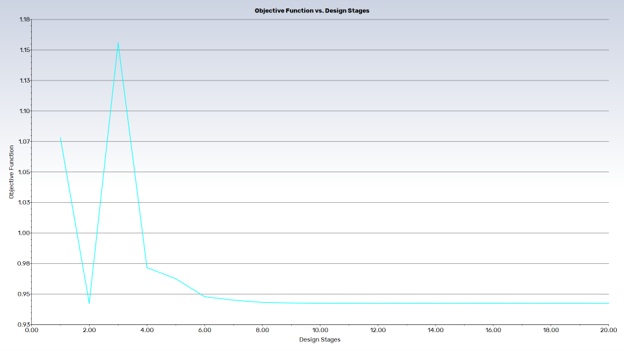
Figure 5: The Powell optimizer was faster, finishing in 20 runs with an objective function of 0.94246775.
Rosenbrock optimizer
Then, we examined the Rosenbrock optimizer. This model takes multiple steps in one direction and changes its speed automatically. If a step is good, it moves faster, but if a step is bad, it turns around and moves slower. In our duct example, this was the slowest method. It needed 50 runs to finish and reached a final objective function of 0.94237756. As you can see in the graph below, it creates very large, sharp spikes during the design stages before it finally finds the right answer.
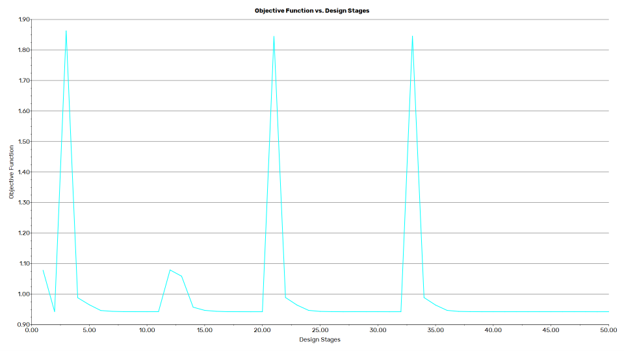
Figure 6: The Rosenbrock optimizer created large spikes and took 50 runs to reach a value of 0.94237756.
Simplex optimizer
Next, we applied the Simplex optimizer. This model uses geometric shapes, like triangles or tetrahedrons, to test the corners of the design. It finds the worst corner and replaces it to improve the flow. This method was the fastest one in our entire test. It only took 14 runs to finish the job. It gave a final objective function of 0.94251924. The graph shows it reached a flat, stable line very quickly compared to all the other models.
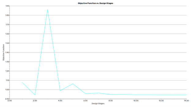
Figure 7: The Simplex optimizer was the fastest method, finishing in only 14 runs with a value of 0.94251924.
Torczon Optimizer
Finally, the Torczon method is an advanced and highly flexible version of the Simplex model. Instead of just flipping the geometric shape, it uses three special mathematical steps: rotation, expansion, and contraction. This flexibility helps it find the optimal design very accurately. Based on our duct case study data, this method completed the optimization smoothly in exactly 24 design stages. Furthermore, it successfully reached the final objective function to 0.94240446.
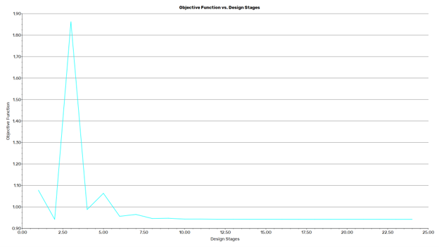
Figure 8: Objective Function vs. Design Stages for the Torczon Optimizer. The method finished in 24 runs with a final objective function of 0.94240446.
To make it very easy for you to choose the best model, we created a short summary table below. We sorted the results from the fastest method to the slowest method. As you can see, all models reached a very similar final objective function around 0.942, but the required time was very different!
Duct System Optimization: Model Performance Table
| Optimizer Model | Total Runs Needed | Final Objective Function | Total Nodes Moved |
| Simplex | 14 runs (Fastest) | 0.94251924 | 6562 |
| Powell | 20 runs | 0.94246775 | 6562 |
| Torczon | 24 runs | 0.94240446 | 6562 |
| Compass | 33 runs | 0.94238611 | 6562 |
| Rosenbrock | 50 runs (Slowest) | 0.94237756 | 6562 |
| NEWUOA | Not Tested | Requires UDF | N/A |
Conclusion
To finalize this report, we must document the physical changes in our optimized geometry to highlight the true effectiveness of the Mesh Morpher. As you can observe in the mesh boundary images below, the tool successfully deformed the initial structure to explore the design space. More importantly, the morphing process perfectly maintained the original mesh topology while precisely adjusting the node locations. Because of this smart node movement, we reached the optimal configuration without any need for repetitive, time-consuming remeshing. When we look at the visual comparison of the “Before” and “After” velocity contours, the quantitative improvements are very clear. The optimized shape successfully reduced the total pressure drop, and the fluid travels through the spiral shape with a much better balance.
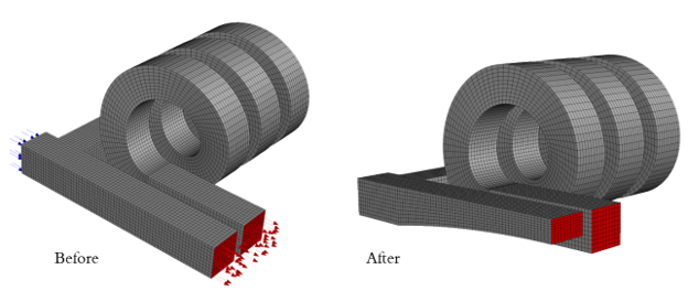
Figure 9: The initial and final computational mesh of our duct geometry. The morphing process maintained this exact topology without requiring a new mesh generation.
Furthermore, the application of the Mesh Morpher resulted in a significantly smoother flow distribution within the helix tube geometry. When dealing with complex curves, moving the walls can sometimes destroy the mesh cells. However, this optimization process effectively mitigated element distortion during the deformation stages. By ensuring that the element quality remained within acceptable limits, the software created a more uniform and stable grid. This smoother distribution inside the helix is essential because it prevents numerical crashes and heavily enhances the final accuracy of the flow simulation.
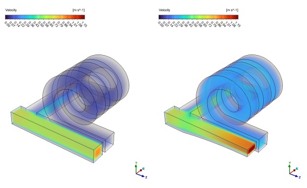
Figure 10: A visual Before and After comparison of the velocity contours. The final optimized geometry shows a smoother, more efficient flow distribution in the helix tube
In conclusion, the Mesh Morpher is a highly reliable and robust tool for engineering shape optimization. Based on our comparison data, the Simplex model was the most efficient method, finishing the task in only 14 runs, while the Rosenbrock model took the longest time. Despite the speed differences, every method successfully improved the geometry using simple direct search math. If you want to test these exact models, check the boundary conditions, and learn the complete setup process yourself, you can get the project files from our Duct System Optimization Tutorial.