
![The Relative Humidity distribution proving water vapor traps in the low-momentum zones, reaching exactly 66.18 [%].](https://cfdland.com/wp-content/uploads/2026/06/RH.webp)

Industrial poultry farms face a massive thermal management problem. Thousands of birds live in a single enclosed space. They release continuous body heat and water vapor. If the airflow fails, the internal temperature and ammonia levels rise rapidly. This creates severe heat stress, which destroys farm productivity. Engineers must design precise tunnel ventilation layouts to remove this heat constantly.
Building physical test structures is far too expensive. In this course, we will solve this HVAC problem using ANSYS Fluent. We will map the exact air velocity, thermal gradients, and moisture concentration inside a commercial broiler house. If you want to master environmental flow physics, studying our HVAC CFD tutorials is your best next step. Today, you will analyze exactly how forced convection physics sweep dangerous thermal loads out of a confined industrial space.
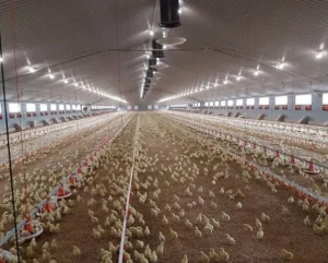
Figure 1: The real internal layout of a commercial broiler house requiring continuous tunnel ventilation for survival.
Simulation Process: HVAC Flow Domain
We define the physical domain using ANSYS SpaceClaim. The geometry represents a long rectangular commercial broiler house. The design features distributed inlet vents along the roof and side walls. A concentrated exhaust fan zone sits at the far end to drive the tunnel ventilation. We process the fluid volume in ANSYS Fluent Meshing. The software generates a high-quality polyhedral mesh containing exactly 2,353,437 poly cells. This dense mesh resolution captures the severe velocity gradients near the inlet jets and the floor boundaries.
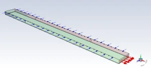
Figure 2: The ANSYS SpaceClaim flow domain defining the distributed roof inlets and the concentrated exhaust boundary.
To capture the complex environmental physics, we activate the Species Transport model. This tracks the exact water vapor concentration to determine the Relative Humidity. We assign precise heat flux boundary conditions along the floor. This represents the continuous metabolic heat generated by the broiler flock. A pressure outlet operates at the exhaust face to pull the internal air volume.
Post-processing
The mass-weighted average report from ANSYS Fluent provides a strict evaluation of the thermal environment. The following table displays the exact performance metrics.
| Parameter | Average Value | Maximum Value |
| Velocity Magnitude | 0.544 [m/s] | — |
| Static Temperature | 32.30 [°C] | 39.58 [°C] |
| Relative Humidity | 59.95 [%] | 66.18 [%] |
The average Velocity Magnitude of exactly 0.544 m/s confirms a successful low-speed forced convection state. The average Static Temperature stays at exactly 32.30°C, which satisfies standard thermal comfort rules for poultry. However, the simulation detected a maximum Static Temperature hitting exactly 39.58°C. This proves that dangerous localized stagnation zones exist. We must now evaluate the spatial distribution data. We will analyze the thermal boundary layers, the fluid momentum of the inlet jets, and the moisture transport physics inside the shed.
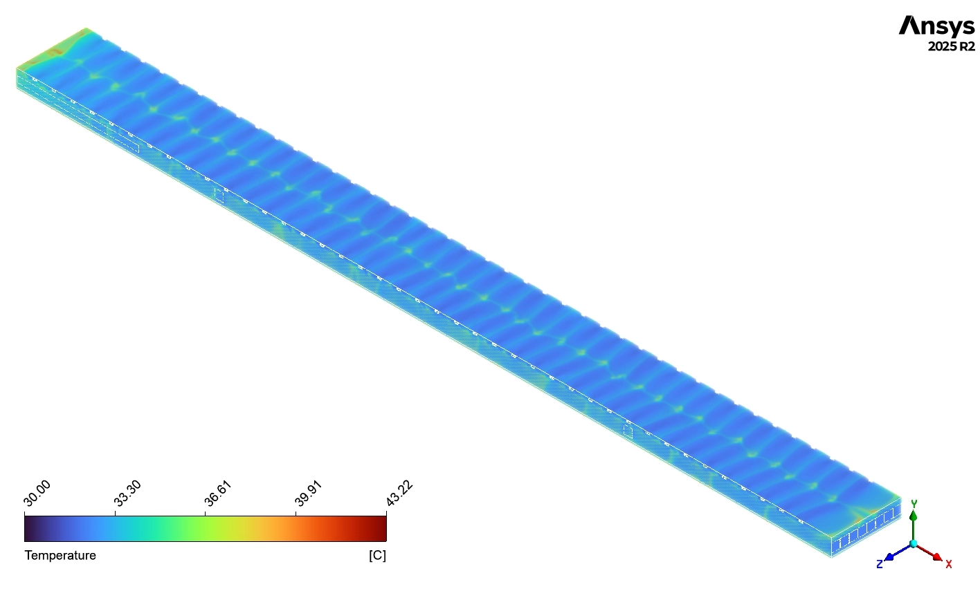
The Surface Temperature contour evaluates the heat transfer through the structure. The data scale shows a dominant distribution range between exactly 30 and 33°C across the main roof and walls. This thermal uniformity proves that the forced tunnel ventilation effectively removes internal heat along the main longitudinal axis. However, the data reveals isolated zones near the inlet corners reaching exactly 36 to 40 [°C]. In fluid mechanics, an incoming fluid jet requires a specific development length before it achieves maximum mixing efficiency. These isolated warm patches exist because the incoming fresh air has not yet developed enough turbulent momentum to strip the boundary layer heat from these specific corners.
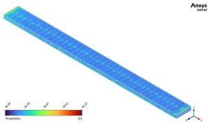
Figure 3: The interior Surface Temperature contour proving the tunnel flow limits structural heating to exactly 33 [°C] on average.
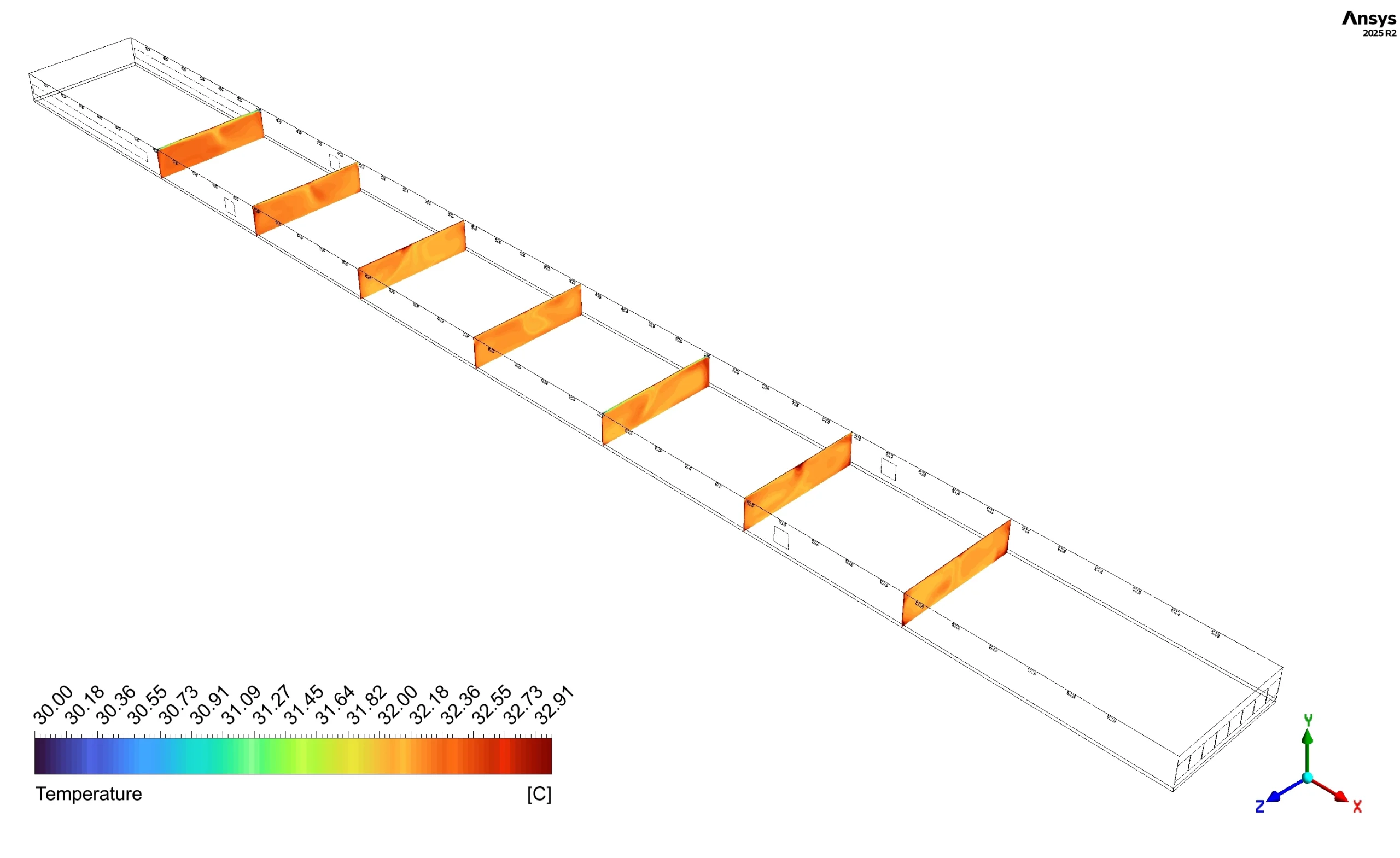
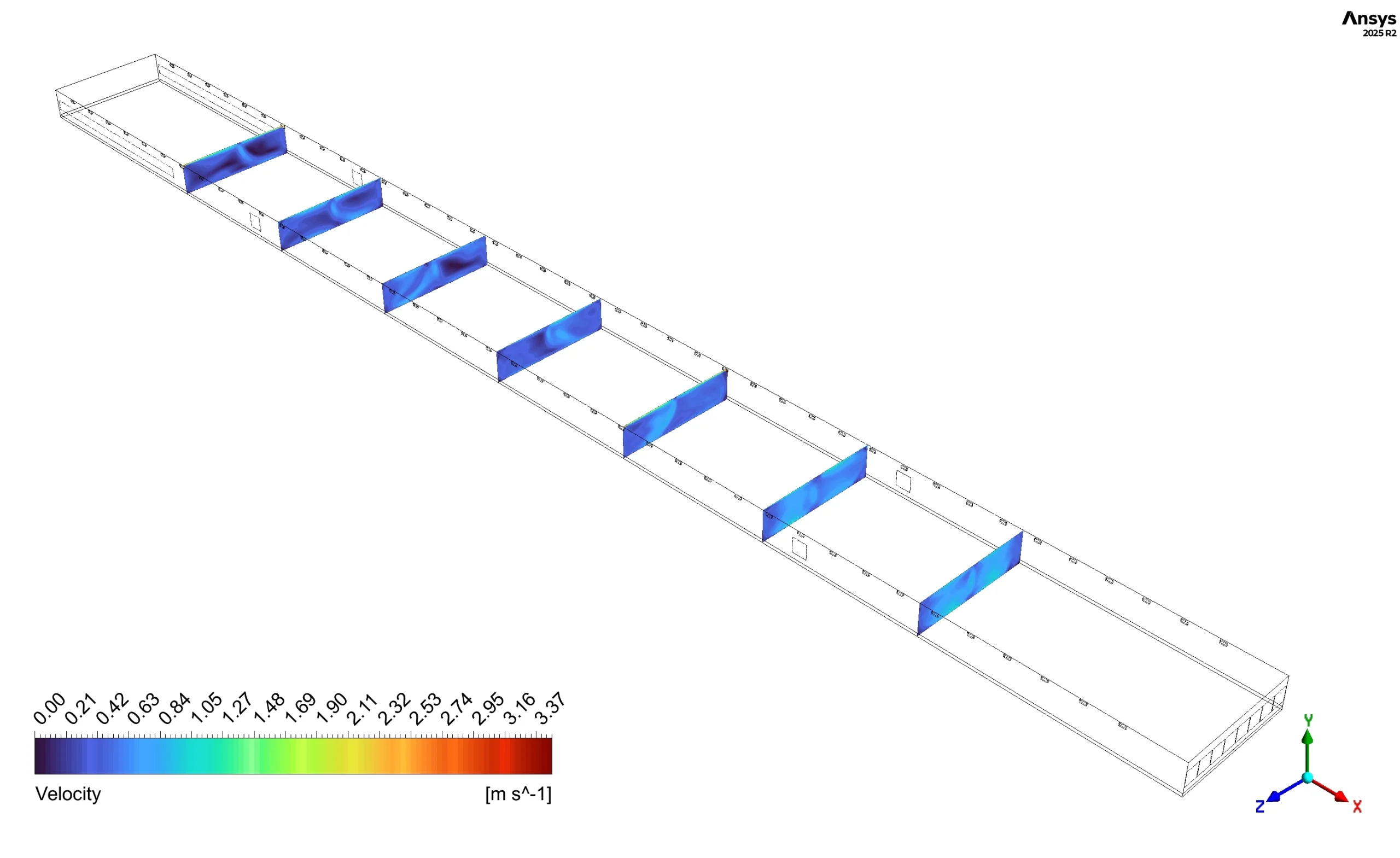
Figure 4 displays the Static Temperature. The spatial distribution shows a strictly uniform range between exactly 30 and 32.91 [°C] on every cross-section. The thermal gradient across all vertical planes remains extremely narrow at approximately 3 [°C]. This is a critical engineering achievement. It proves that severe thermal stratification does not occur. The heat flux generated at the floor boundary mixes thoroughly with the upper air volume. The longitudinal airflow successfully transports the thermal load downstream without allowing heat to accumulate violently inside any single intermediate bay.
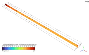
Figure 4: The internal cross-sections proving the forced convection prevents severe thermal stratification between the floor and ceiling.
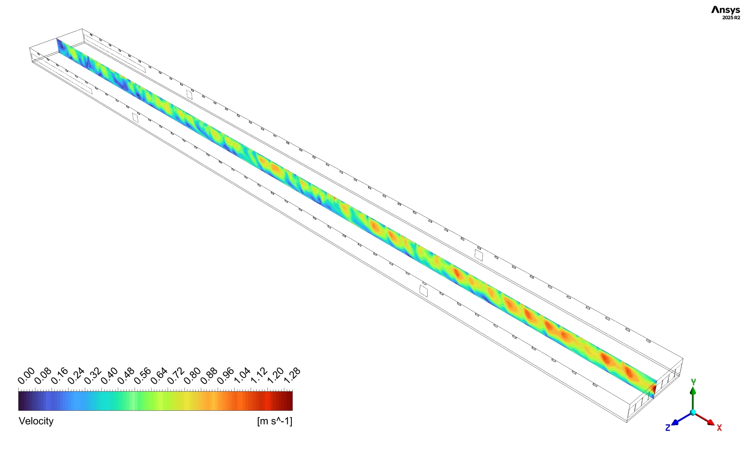
Figure 5 maps the Velocity Magnitude using fluid pathlines. The physical inlet jets inject fresh air at high momentum, reaching a maximum velocity of exactly 3.70 m/s. As these jets enter the large internal volume, they expand and lose momentum. This expansion forces the air to roll into large recirculating loops inside each bay. These loops operate between exactly 0.37 and 1.11 m/s. This recirculation physics drives the primary mixing mechanism. It forces the fresh ceiling air down to the floor level.
However, the pathlines reveal critical stagnation zones at the floor leve. The velocity here drops to exactly 0m/s. Because the fluid lacks momentum, the air exchange rate fails completely. These dead zones trap the metabolic heat, directly causing the maximum localized Static Temperature of exactly 39.58 °C reported in the data table.
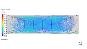
Figure 5: The Velocity Magnitude pathlines revealing high-momentum jets hitting exactly 3.70 [m/s] and critical zero-velocity dead zones.
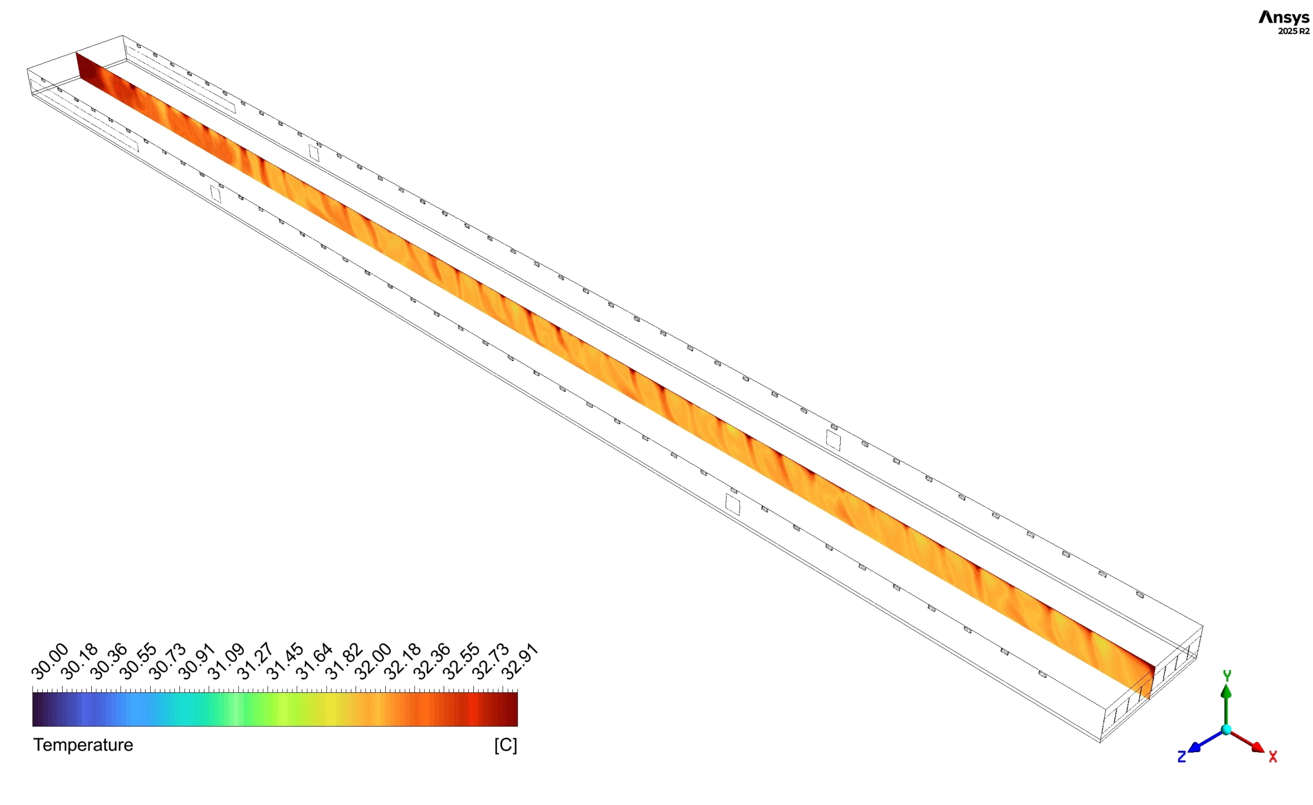
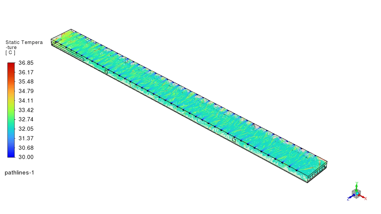
Figure 6 shows the 3D Static Temperature pathlines tracking the total mass transport. The inlet air enters the domain at exactly 30 to 31 °C. As the fluid sweeps over the floor boundary, forced convection transfers the metabolic heat into the air stream. The fluid temperature rises steadily along the longitudinal axis, eventually reaching exactly 36.85 °C at the exhaust boundary.
The center-plane contour confirms that a narrow thermal corridor running between exactly 31 and 32.91 °C dominates the centerline. The sidewall zones remain cooler at exactly 30 to 30.55 °C. The central flow channel carries the highest momentum and the highest thermal load.
Figure 7 evaluates the Relative Humidity calculated by the Species Transport model. The moisture concentration follows the exact same transport physics as the heat. Because the central tunnel flow is highly efficient, the average humidity remains stable. However, the lack of momentum in the peripheral stagnation zones causes water vapor to accumulate, pushing the local maximum Relative Humidity to an dangerous limit of exactly 66.18 [%]. This specific CFD data commands engineers to reposition the inlet vents to eliminate these peripheral dead zones.
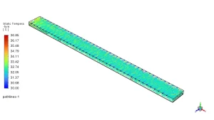
Figure 6: The 3D Static Temperature flow path proving the continuous forced convection transfers the thermal load to the exhaust.
![The Relative Humidity distribution proving water vapor traps in the low-momentum zones, reaching exactly 66.18 [%].](https://cfdland.com/wp-content/uploads/2026/06/RH-300x169.webp)
Figure 7: The Relative Humidity distribution proving water vapor traps in the low-momentum zones, reaching exactly 66.18 [%].
Frequently Asked Questions (FAQ)
- Why does tunnel ventilation prevent severe thermal stratification?
- Tunnel ventilation creates continuous forced convection. The high-momentum inlet jets generate large recirculation loops. These loops physically force the fresh upper air to mix with the dense, hot air near the floor, equalizing the temperature across the vertical plane.
- What causes localized stagnation zones in a commercial shed?
- Fluid streams lose momentum as they expand into large volumes. When the structural baffles disrupt the main airflow path, the fluid velocity behind the obstacles drops to zero. Without velocity, convective heat transfer stops completely.
- How does the Species Transport model evaluate Relative Humidity?
- The Species Transport model tracks the precise mass fraction of water vapor inside the air mixture. By calculating the local static temperature, absolute pressure, and exact vapor concentration, ANSYS Fluent determines the exact local relative humidity percentage.


Reviews
There are no reviews yet.