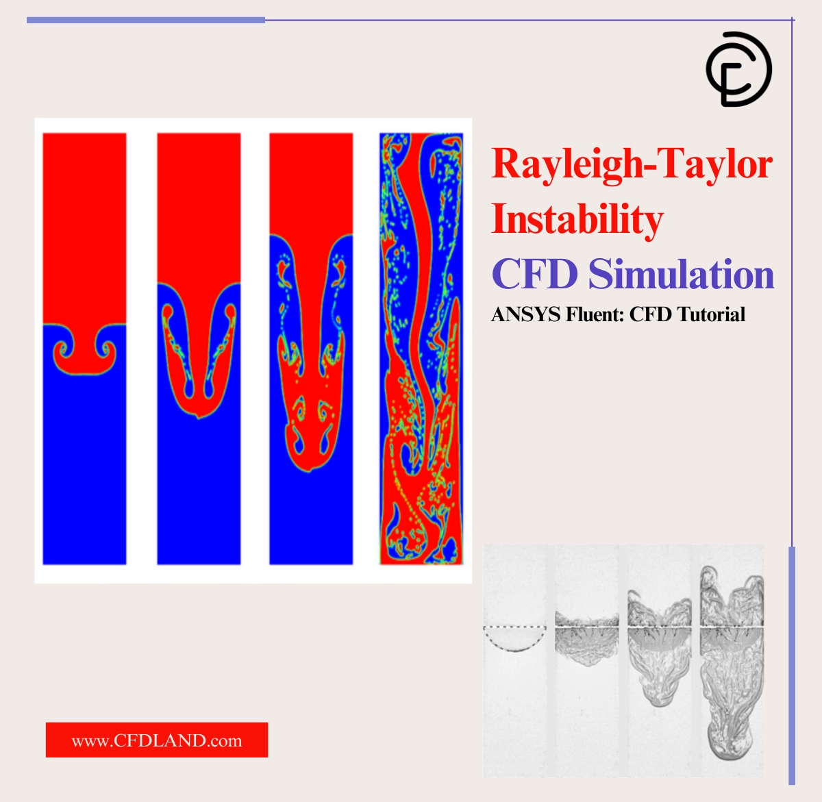
Placing a heavy fluid directly on top of a light fluid creates a severe structural imbalance. Gravity constantly pulls the heavy fluid downward. The light fluid resists and attempts to rise. This interaction creates a highly volatile boundary. A microscopic vibration will cause the boundary to collapse violently. Engineers define this collapse as the Rayleigh-Taylor instability. Predicting exactly how these fluids tear apart and mix is a critical challenge in aerospace, chemical reactors, and astrophysics.

Replicating this precise chaotic mixing in a physical laboratory is extremely difficult. Therefore, engineers solve this problem using ANSYS Fluent. We utilize the multiphase solver to track the exact deformation of the fluid interface over time. If you want to master complex liquid interactions, exploring our Multiphase CFD tutorials is your best next step. Today, you will analyze exactly how a tiny surface wave transforms into a massive turbulent mixing field under pure gravitational acceleration.

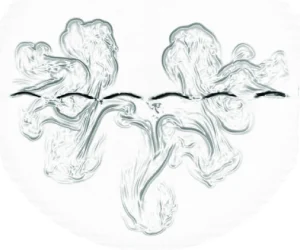
Figure 1: Experimental investigation of two-dimensional Rayleigh-Taylor instability with controllable initial conditions

Simulation process: Multiphase Perturbation Setup

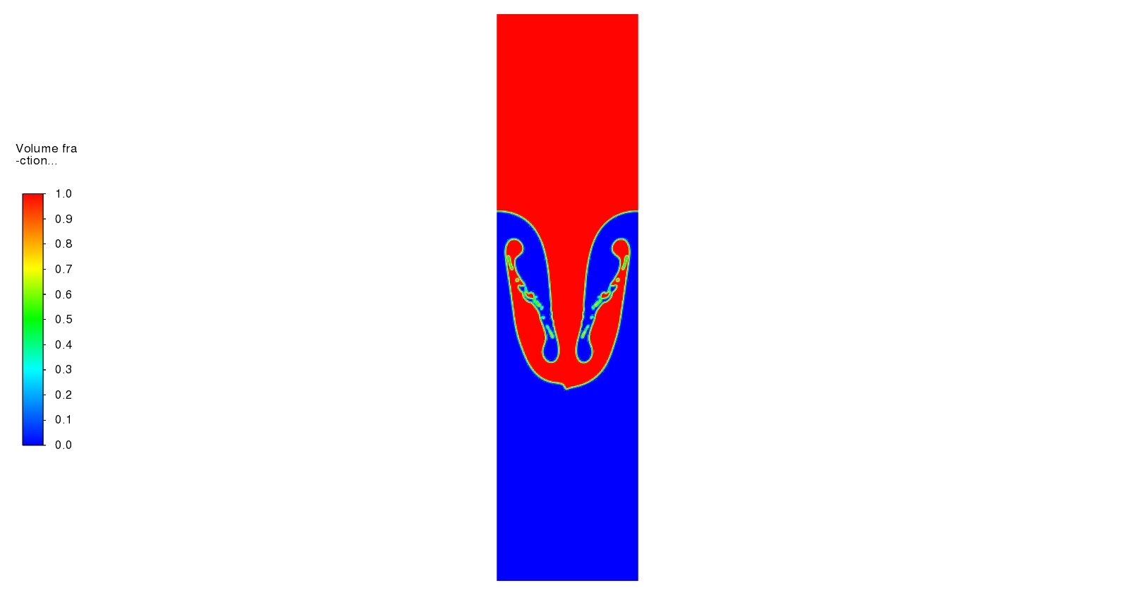
To capture the true physics of the instability, we must initiate a controlled mathematical imbalance. We configure a two-dimensional domain containing two distinct fluid phases. We place the heavy fluid at the top and the light fluid at the bottom. We activate the Volume of Fluid model to track the sharp density boundary.

We cannot rely on random numerical errors to start the mixing. We must write an ANSYS Fluent User-Defined Function(UDF) to force a specific geometric wave at the interface. We apply a cosine wave perturbation exactly at a mean height of 0.5. We assign this wave a strict amplitude of 0.05 and a wavelength of 0.25. This mathematically perfect initial condition forces the gravitational instability to grow symmetrically.

Post-processing: Analysis of Multiphase Mixing

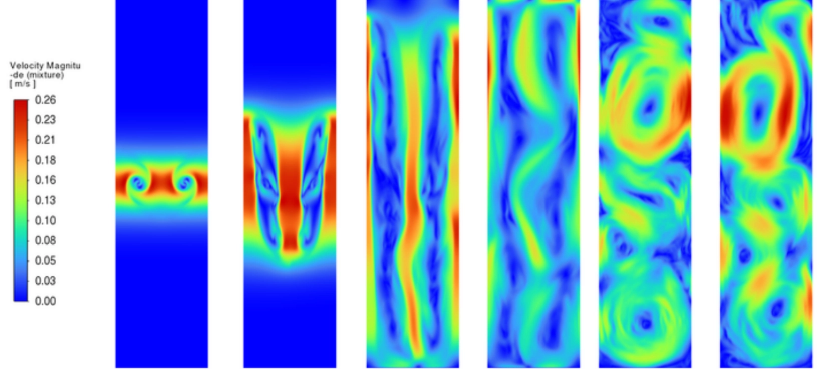
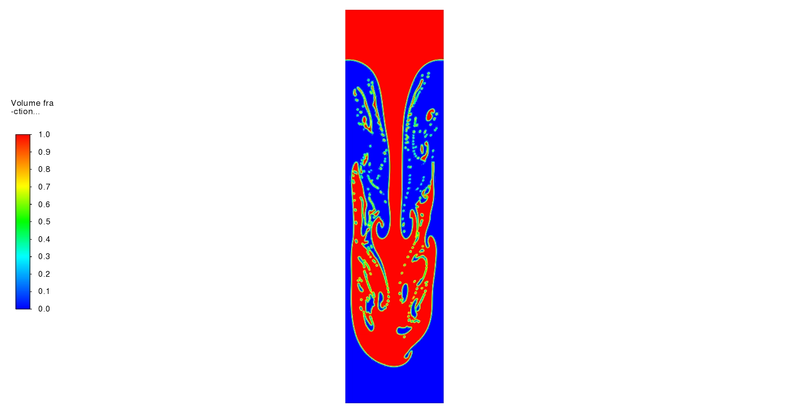
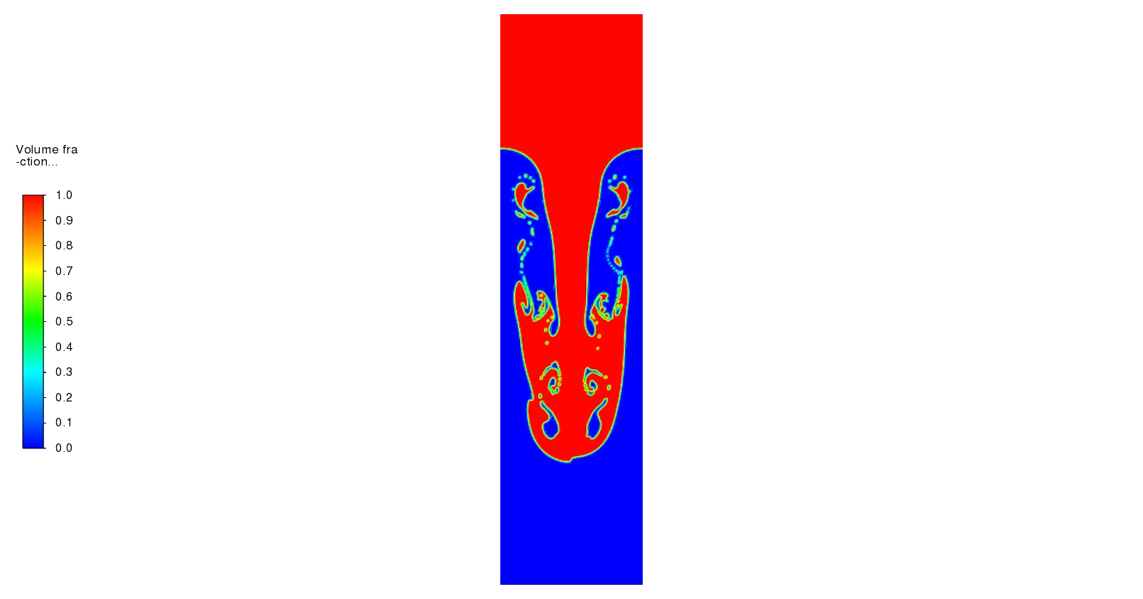
The transient evolution of this multiphase flow reveals a strict sequence of fluid dynamics. We begin by examining the initial growth phase visible in the first transient frames. The mathematical cosine perturbation instantly triggers the gravitational imbalance. The heavy fluid begins to accelerate downward, forming distinct vertical columns called spikes. Simultaneously, the displaced light fluid accelerates upward, forming rounded structures called bubbles. During this early linear growth phase, the maximum velocity magnitude concentrates exclusively along the edges of these moving structures, hitting the initial peak of 0.26 m/s. The surrounding fluid mass far above and below the interface remains completely stationary. This isolated momentum proves that the initial motion is driven entirely by local density variations and gravitational body forces, exactly as the mathematical theory predicts.

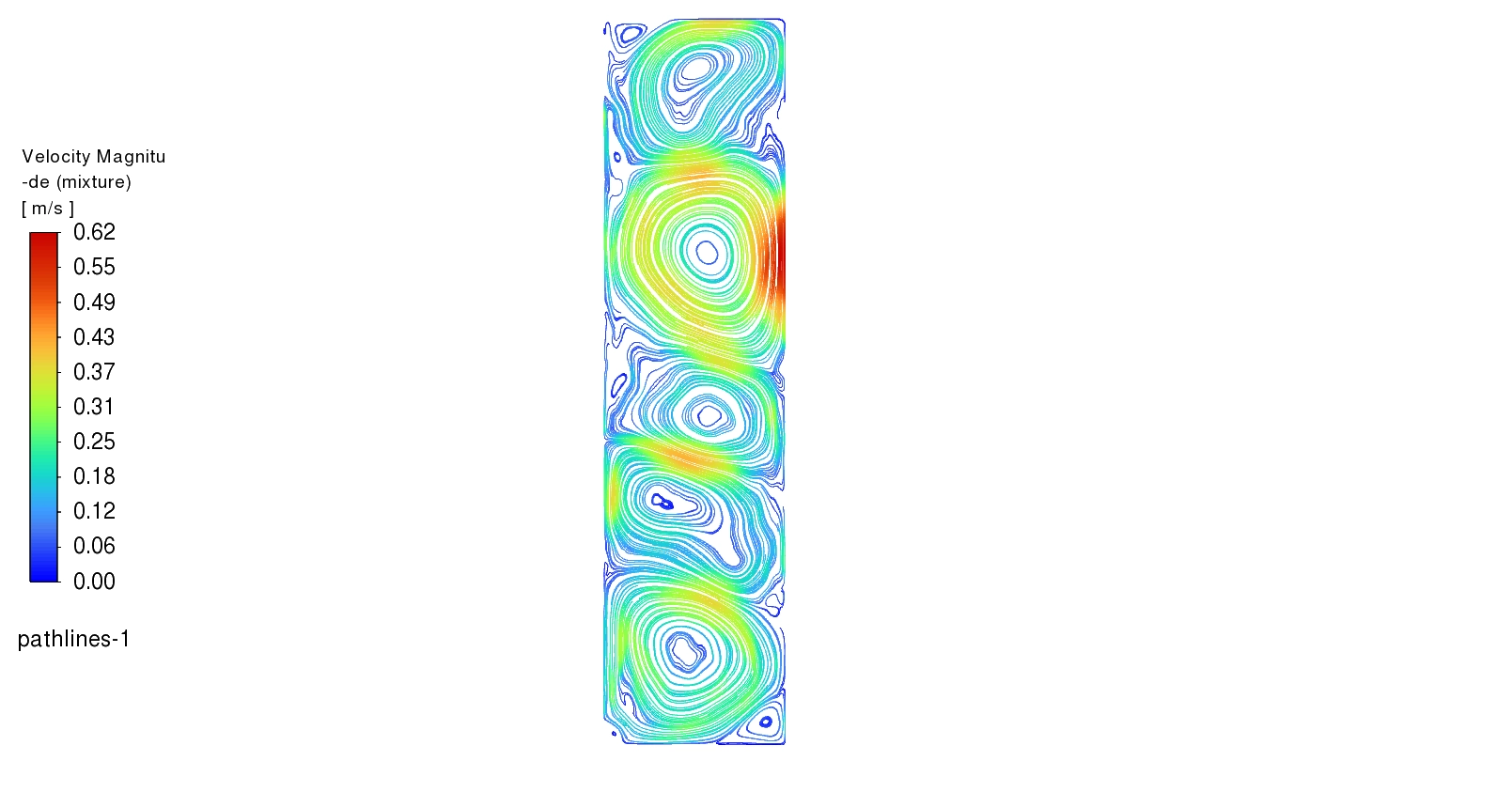
As time advances, the physics enter a highly violent nonlinear phase. The falling heavy spikes gain massive downward momentum. As these heavy spikes shear against the rising light bubbles, extreme friction occurs along the fluid boundary. This intense shear force generates secondary aerodynamic instabilities. The straight downward flow breaks apart. The velocity streamlines reveal the exact formation of massive, counter-rotating vortices. The fluid begins to spin rapidly around the falling spikes. This intense rotational momentum acts as a fluid centrifuge, driving the localized velocity to an extreme peak of 0.62 m/s. The flow completely loses its initial vertical symmetry. The straight pathlines collapse into tight circular loops, proving that sheer forces have overpowered the simple gravitational drop.

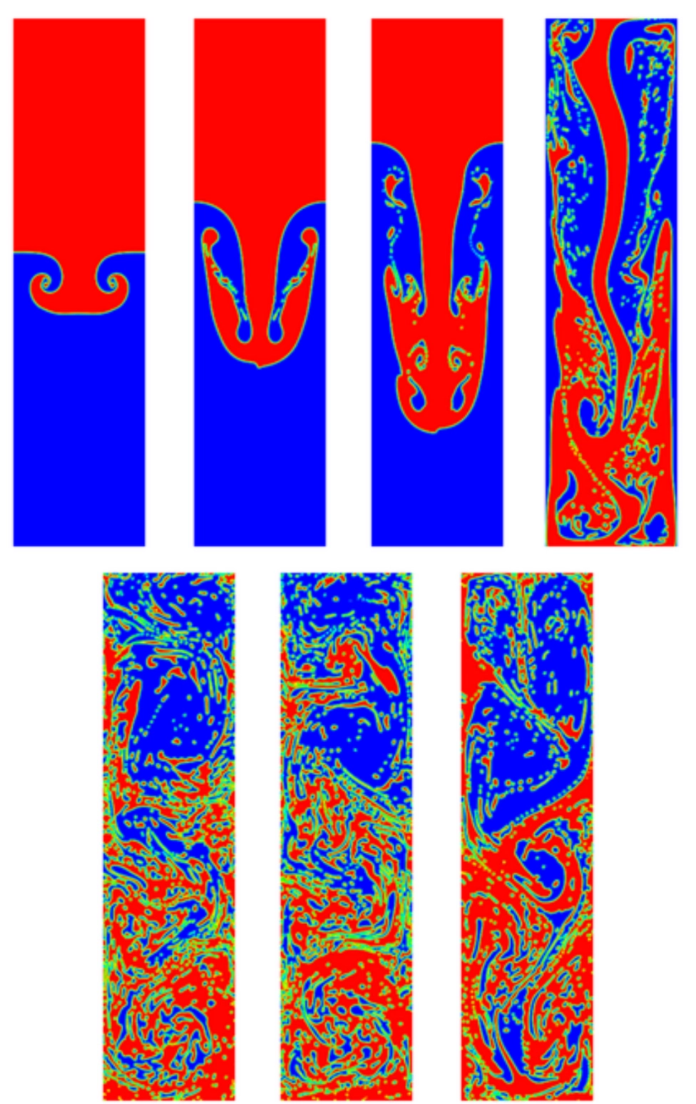
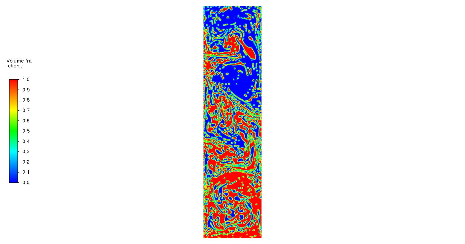
Figure 2: The transient multiphase tracking proving the falling heavy spikes and rising bubbles physically shred into a chaotic turbulent mixture.

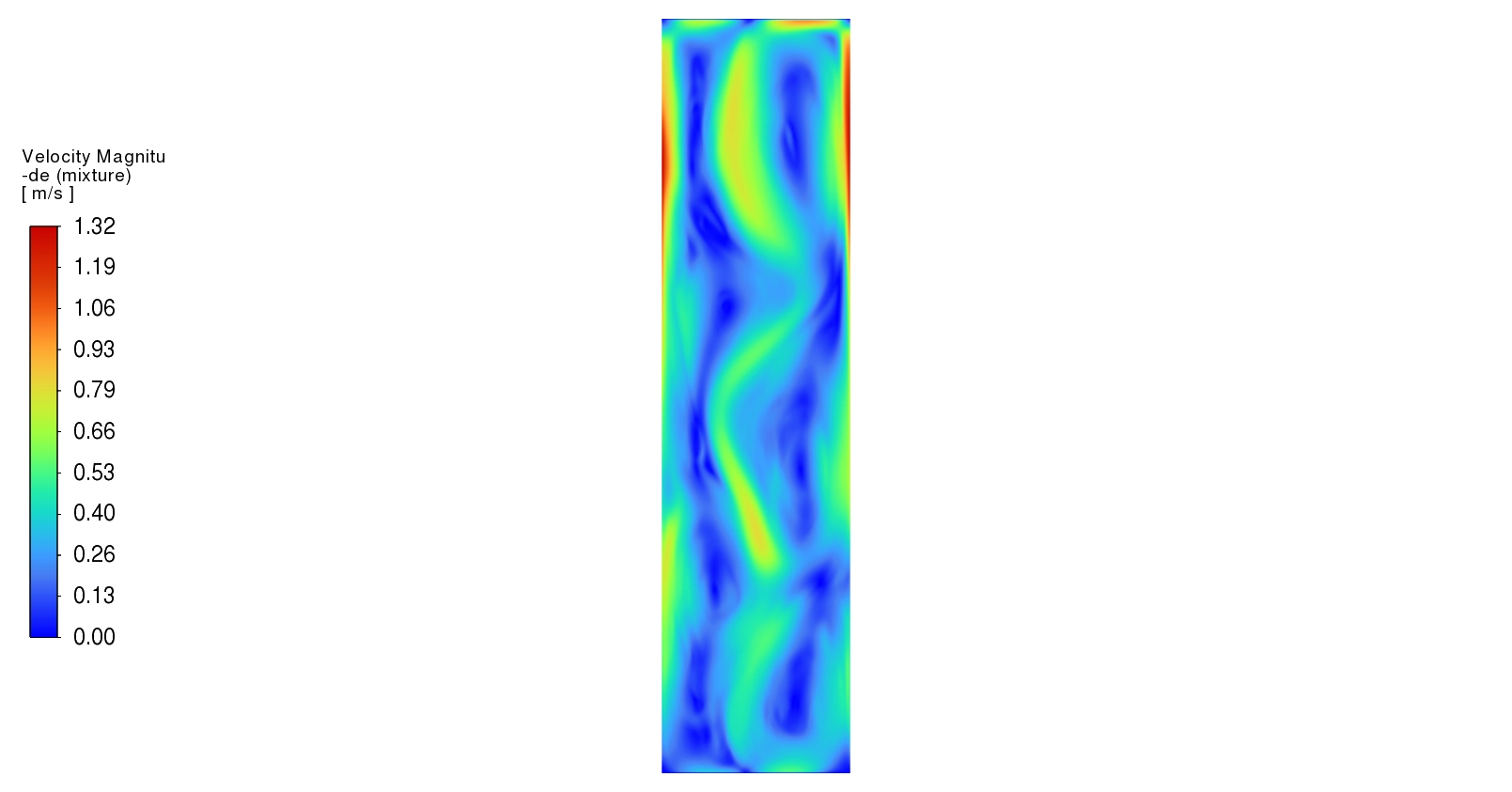
Figure 3: The transient velocity evolution proving the initial interface momentum transitions into a disorganized turbulent flow field.

In the final transient stages, the entire flow domain surrenders to chaotic turbulent mixing. The distinct structural boundaries of the spikes and bubbles cease to exist. The intense rotational vortices physically shred the fluid interface. The heavy fluid rips apart into disconnected droplets and chaotic filaments. This rapid shredding is a direct result of the Kelvin-Helmholtz instability acting upon the edges of the Rayleigh-Taylor spikes. The global velocity field scatters unpredictably across the entire domain, settling into a disorganized range between 0.08 m/s and 0.26 m/s. The Volume of Fluid contours prove that the two separate density phases have achieved profound mechanical blending. This final chaotic state confirms that the multiphase solver successfully resolved the complete life cycle of the instability, transforming a simple mathematical surface wave into a fully turbulent multiphase mixture.

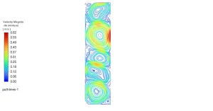
Figure 4:  The velocity pathlines revealing the massive counter-rotating vortices created by severe shear forces at the fluid boundaries.

Frequently Asked Questions (FAQ)

• What triggers the Rayleigh-Taylor instability?
  • The instability requires two conditions. First, a dense fluid must rest on top of a lighter fluid. Second, a gravitational acceleration must act upon them. Because the heavy fluid wants to sink and the light fluid wants to rise, any microscopic disturbance at their boundary will cause them to penetrate each other violently.
• Why do counter-rotating vortices form during the mixing?
  • As the heavy fluid falls, it rubs directly against the rising light fluid. This opposite motion creates severe shear stress along the vertical boundary. This intense friction physically rolls the fluid edges into spinning vortices, which rapidly destroy the structural shape of the falling spikes.
• Why is a User-Defined Function necessary for the setup?
  • To study the exact mathematical growth rate of the instability, engineers cannot rely on random numerical noise to start the mixing. The User-Defined Function injects a perfectly calculated geometric wave into the interface. This forces the fluid to mix in a predictable, symmetrical pattern that can be validated against pure physics equations.